Download
1 / 19
190 likes | 361 Views
Monitoring Tropospheric Ozone from Ozone Monitoring Instrument (OMI). Xiong Liu 1,2,3 , Pawan K. Bhartia 3 , Kelly Chance 2 , Thomas P. Kurosu 2 , Robert J.D. Spurr 4 , Bojan R. Bojkov 1,3 , Ozonesonde Providers xliu@umbc.edu 1 Goddard Earth Sciences and Technology Center,UMBC

E N D
Monitoring Tropospheric Ozone from Ozone Monitoring Instrument (OMI) Xiong Liu1,2,3, Pawan K. Bhartia3, Kelly Chance2, Thomas P. Kurosu2, Robert J.D. Spurr4, Bojan R. Bojkov1,3, Ozonesonde Providers xliu@umbc.edu 1Goddard Earth Sciences and Technology Center,UMBC 2Harvard-Smithsonian Center for Astrophysics 3NASA Goddard Space Flight center 4RT Solutions Inc. 7th CMAS Conference Chapel Hill, North Carolina, October 7th, 2008
Outline • Introduction • Retrieval algorithm, information content and retrieval errors • Comparison of OMI ozone profiles and stratospheric ozone column with MLS data • Comparison of OMI ozone profiles and tropospheric ozone columns with ozonesonde data • Examples of retrieved tropospheric ozone • Summary Show that the use of OMI ozone profiles as boundary conditions can significantly improve the CMAQ simulations. Pour Biazar (oral) Wang (poster)
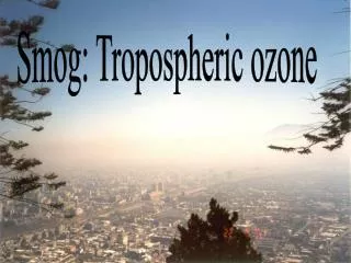
Introduction • Backscattered Ultraviolet (BUV) technique [Singer&Wentworth, 1957]: • Measure ozone profiles since the 1970s (BUV, SBUV, SBUV2) • Provide little information below 25 km [Bhartia et al., 1996]. • Tropospheric O3 Column (TOC): total O3-strat. O3 column (SOC) • Poor spatiotemporal sampling (e.g., low vertical resolution of nadir sensors and poor horizontal sampling of limb sensors) or large uncertainty in SOC • Most methods only derive monthly mean TOC in the tropics • With advanced instrumentation (OMI/MLS on AURA) and techniques (e.g., PV/trajectory mapping, assimilation), possible to derive daily TOC globally [Yang et al., 2007, Schoeberl et al., 2007; Stajner et al., 2007] • Tropospheric O3 retrievals from hyper-spectral UV instruments (e.g., GOME, OMI) [Chance et al.,1997, Munro et al.,1998, Liu et al., 2005] • Strong wavelength dependence of ozone absorption in the Hartley and Huggins bands coupled with wavelength-dependent Rayleigh scattering • Temperature dependence in the Huggins bands (313-340 nm) • We developed an 8-year (July 1995-June 2003) dataset of GOME ozone profiles and are applying our algorithm to OMI data
Introduction • OMI [Levelt et al., 2006]: • Nadir-viewing UV/Visible instrument (270-500 nm) • Spatial resolution of 13×24 km2 at nadir & daily global coverage • OMI ozone profile retrieval [Liu et al., 2005] • Retrieve ozone at 24 ~2.5-km thick layers from surface to ~60 km using 270-330 nm radiances • Optimal estimation technique [Rodgers, 2000] • Use ozone profile climatology by Mcpeters et al. [2007] to constrain retrievals
In practice, due to instrumental calibration error and inadequate forward modeling (e.g., aerosols, clouds), the information retrieved in the lower troposphere is significantly reduced. Retrieval Averaging Kernels • DFS: 5-8 with up to 1.5-2 in the troposphere. • Vertical resolution: ~6-8 km FWHM in the stratosphere and ~10 km in the troposphere • AKs for the bottom layer peak at this altitude. • Trop. O3 info. decreases with latitude and solar zenith angle
Random (N) and Smoothing (S) Errors • Random Errors (N): <~2% above 22 km and within ~10% below • Smoothing+Random Errors: within 3% between 22-40 km, increase to 10% above 40 km, and to 20-30% below 20 km. • Errors in O3 columns (SZA < 85º) • Stratospheric O3 column: 1-2.5 DU (N), 2-5 DU (S+N) • Tropospheric O3 column: 1-3 DU (N), 2-6 DU (S+N) • Total O3 column: 0.3-2 DU (N), 0.5-4 DU (S+N)
Comparison with MLS Ozone Profiles • MLS: on-board EOS-AURA, spatiotemporally coincident with OMI • MLS O3 error estimate:~5% in the strat., ~10-15% in the lower strat., ~2-3% in stratospheric O3 column [Froidevaux et al., 2007] • OMI agrees well with MLS to within their uncertainties With OMI AKs
Comp. with MLS 215 hPa O3 Column • Mean bias(2006) • -0.65±2.75% (-1.8 ±7.6 DU) • O3 column above 215 hPa can be accurately derived from OMI data alone !!!
Comparison with Ozonesondes • Ozonesonde data: available at AURA AVDC for August 2004-March 12, 2008 • Coincidence criteria: within 6 hours, 1º lon./lat., cloud fraction (<0.3) • Focus on two latitude bands with enough coincidences: 30ºS-30ºN, 30ºN-60ºN • Compare profile and tropospheric O3 columns (surface-200 mb, surface-~5km, surface-~2.5km) • Ozonesonde profiles are convolved with OMI averaging kernels, but not the tropospheric ozone columns
Comparison with Ozonesondes (30ºS-30ºN) Solid line: mean Dashed line: 1 • Profile: within 10%, significant improvement throughout the troposphere
Comparison with Ozonesondes (30ºS-30ºN) Sfc-200mb Sfc-~5km • Sfc-200 mb: –0.34.9 DU, (r=0.84), slope=0.73 • Sfc-~5 km: –0.23.5 DU, (r=0.76), slope=0.64 • Sfc-~2.5 km: –0.22.4 DU, (r=0.69), slope=0.49 Sfc-~2.5km
Spring Winter Summer Fall Comparison with Ozonesondes (30ºN-60ºN) • Within 10-30%, improvement in the middle and upper troposphere. • Seasonal dependent biases.
Comparison with Ozonesondes (30ºN-60ºN) Sfc-200mb Sfc-~5km • Winter: 2.87.9 DU, R = 0.65 • Spring: 2.97.3 DU, R = 0.75 • Summer: -1.65.4 DU, R = 0.79 • Fall: 1.45.2 DU, R = 0.62 Sfc-~2.5km
First Layer (0-3 km) Ozone over Southeast Asia 2005m1013 2006m1021 • Enhanced ozone over Indonesia in Oct. 2006 relative to Oct. 2005. • Enhanced ozone over South China especially in Oct. 2006.
Column-Averaged O3 Mixing Ratio (July 15 – September 7, 2006)
Summary • Stratospheric and tropospheric O3 columns can be well derived from OMI alone. • OMI O3 profiles and stratospheric O3 column compare well with MLS, to within combined retrieval uncertainties. • OMI O3 profiles and tropospheric O3 columns generally compare well with sondes, but show seasonal/lat./alt.-dependent biases. • Retrieved tropospheric ozone can capture some signals due to pollution, biomass burning, regional and intercontinental transport, convection, and stratospheric influence. • Our product is currently a reseach product and we plan to make it an operational product. • Acknowledgements • OMI and MLS Science Teams • Support from NASA • Support from various organizations on ozonesonde observations
“Boundary ozone” (0-2.5 km) Ozone over Southeast Asia 2005m10 2006m10 • Enhanced ozone over Indonesia in Oct. 2006 relative to Oct. 2005. • Enhanced ozone over South China especially in Oct. 2006.
Comparison with Ozonesondes (30ºS-30ºN) Sfc-~5km A Priori W/O OMI AKs With OMI AKs
Comparison with Ozonesondes (30ºN-60ºN) Sfc-~5km A Priori W/O OMI AKs With OMI AKs