Evaluating the Role of Confounding

1. Evaluating the Role of Confounding

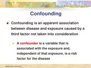
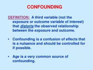
2. Definition and Impact • An alternate explanation for an observed association between an exposure and disease. • A mixing of effects. • association between exposure and disease is distorted because it is mixed with the effect of another factor that is associated with the disease. • Confounding distorts the true association.

3. An Example: Who can run faster, men or women? • Exposure = gender • Outcome = speed • Null Hypothesis • average speed of men = average speed of women • All men and women in one town invited to participate in a road race. On race day, both men and women come and race. The average running time for the men is faster than the women. • CONCLUSION: Men run faster than women because of their gender.

4. An Example: Who can run faster, men or women? • But wait! Someone notices that women with young children did not race. In fact, women who ran the race were, on average, older than men who ran. For example, the average age of women was 50 years while the average age of men was 25 years. • CONCLUSION: Perhaps men were faster not because of their gender, but because they were younger.

5. An Example: Who can run faster, men or women? • So another race is held, this time making sure ages in the two compared groups (men and women) are comparable. That is, the men and women have same distribution of ages. • Race result: Once again, men are faster. • CONCLUSION: Controlling for age, men are still faster than women.

6. An Example: Who can run faster, men or women? • BUT WAIT! Someone points out that the men are, on average, taller than the women. • CONCLUSION: Perhaps men were faster not due to their gender, but because their legs are longer. • So another race is held, this time making sure heights and ages in the two groups (men and women) are comparable. • Race result: Once again, men are faster.

7. An Example: Who can run faster, men or women? • BUT WAIT! Someone points out that 50% of the women had hair longer than their shoulders, and only 5% of the men did! • CONCLUSION? Long hair made the women run slower. • Is this a reasonable conclusion?

8. Lessons from the road race: Criteria for a characteristic to be a confounder • For a characteristic to be a potential confounder, it must be associated with both the disease (outcome) and the exposure under study. • Exposure  gender • Outcome  race time • Why are age and height competing explanations, but not hair length?

9. Criteria for a Characteristic to be a Confounder • Must be associated with disease independently of exposure. • Example: Age and height are associated with speed regardless of gender. • Taller people have greater speed • Younger people have greater speed. • Is short hair associated with greater speed? • Can test whether a potential confounder is associated with the outcome in non-exposed.

10. Criteria for a Characteristic to be a Confounder • Must be associated with the Exposure • Example: In this example age and height are associated with being male. • Taller people are more likely to be male • Younger people are in this example were more likely to be male. • Is short hair associated with being male -- yes • Why you want exposed and unexposed to be similar in a cohort study. • Why we randomize.

11. Criteria for a Characteristic to be a Confounder • A variable cannot be a confounder if it is a step in the causal chain or pathway. • See next slide for example of step in causal chain

12. Criteria for a Characteristic to be a Confounder Exposure  Disease Moderate Alcohol Consumption (E)  Decreased CHD (D) • Increased HDL (C)  Decreased CHD (D) • Alcohol Consumption (E)  Increased HDL (C) Is HDL a confounder or not?

13. Criteria for a Characteristic to be a Confounder Exposure  Disease Moderate Alcohol Consumption Increased HDL  Decreased CHD Is HDL a confounder or not? NO … It is a step in the causal chain

14. Criteria for a Characteristic to be a Confounder Exposure  Disease Diabetes (E)  CHD (D) Obesity (C)  CHD (D) Obesity (C)  Diabetes (E) Is Obesity a confounder or not?

15. Criteria for a Characteristic to be a Confounder Exposure  Disease Obesity(C?) Diabetes (E)  CHD (D) Is Obesity a confounder or not? Depends – • Is obesity associated with CHD independent of Diabetes, or is obesity associated with CHD only because it causes diabetes? • Is obesity associated with CHD in those without diabetes? • Adjusting for obesity is likely over controlling because obesity increases the risk of diabetes.

16. Cases of Down Syndrome by Birth Order ( Main Exposure) EPIET (www)

17. Cases of Down Syndrome by Age Groups (confounder?) Is age associated with down syndrome? Is age associated with birth order? EPIET (www)

18. Cases of Down Syndrome by Birth Order and Maternal Age EPIET (www)

19. Confounding • A third factor which is related to both exposure and outcome, and which accounts for some/all of the observed relationship between the two. • Confounder nota result of the exposure • Age is a confounder of the association between birth order and down syndrome. • Age is associated with the exposure – birth order • Age is independently associated with the outcome – down syndrome

20. Confounding To be a confounding factor, two conditions must be met: Exposure Outcome Third variable Be associated with exposure - without being the result of exposure Be associated with outcome - independently of exposure (not an intermediary)

21. Confounding Birth Order Down Syndrome Maternal Age Maternal age is correlated with birth order and a risk factor even if birth order is low

22. Is Maternal Age a Confounder ? Down Syndrome Maternal Age Birth Order • Birth order is not associated with down sydrome in young mothers. Maternal Age is not on the causal pathway between birth order and down sydrome. • Age confounds the relationship between birth order and down syndrome

23. Is smoking a confounder? Coffee CHD Smoking Smoking is correlated with coffee drinking and a risk factor even for those who do not drink coffee

24. Confounding ? Smoking Coffee CHD Coffee drinking may be correlated with smoking but does not cause smoking. Smoking is associated with CHD in those who don’t drink coffee. Smoking is not on the causal pathway between coffee and CHD. Smoking confounds relationship between coffee and CHD

25. Confounding Alcohol Lung Cancer Smoking Smoking is correlated with alcohol consumption and a risk factor even for those who do not drink alcohol

26. Confounding ? Smoking CHD Yellow fingers Not related to the outcome Not an independent risk factor Yellow fingers not a confounder

27. Confounding ? Diet CHD Cholesterol On the causal pathway

28. Confounding ? Alcohol CHD HDL Cholesterol On the causal pathway

29. Confounding Randomisation, matching and restriction can be tried at the time of designing a study to reduce the risk of confounding. At the time of analysis: Stratification and multivariable (adjusted) analysis can achieve the same. Which is preferable?

30. Effect of randomisation on outcome of trials in acute pain Bandolier Bias Guide (www)

31. Confounding Obesity Mastitis Age In cows, older ones are heavier and older age increases the risk for mastitis. This association may appear as an obesity association

32. Confounding – Age is the confounder. If each case is matched with a same-age control, there will be no association (OR for old age = 2.6, P = 0.0001) (www)

33. Criteria for a Characteristic to be a Confounder • Examples of confounding • Smoking is confounder of effect of occupational exposures (to dyes) on bladder cancer • Those exposed to dyes are more likely to smoke. • Smoking is an independent risk factor for bladder cancer. • Age is confounder of effect of DDT pesticide exposure and breast cancer • Older people are more likely to have exposure to DDT. • Older people are more likely to have breast cancer.

34. Why Control for Confounding, in General • Confounding factors are nuisance variables. • They get in the way of the relation you want to study. • You want to remove their effect. • We have done this already in age-standardization • You can control in the design or analysis phase.

35. Controlling for Confounding, in General • Which variables are potential confounders? • Usually, risk factors for disease. • Is a variable a confounder in your data or not? • Stratified analysis -- one way, cow example • Compare crude and adjusted measures of association. • If they differ appreciably, the answer is “yes.” • But you may be over controlling.

36. Controlling for Confounding in the Analysis: Stratification TOTAL DATA (One 2 x 2 Table) Crude OR = 2.2

37. Stratified Data (Two 2 x 2 Tables) Age< 40 Age 40 and over Stratum-specific OR = 2.8 Stratum-specific OR = 2.8 Note each stratum is like a restricted analysis. There is a narrow range of the confounder. The stratum specific ORs (2.8) differ from the crude OR (2.2) by about 25%. This difference indicates that there is confounding by age.

38. Controlling for Confounding in the Analysis: Stratification • Pooling stratum specific estimate into one estimate: various methods including the Mantel-Haenszel method. • What if stratum-specific estimates are appreciably different? This is effect measure modification (see Chapter 14, for more details). • Definition of effect measure modification: when magnitude of effect of an exposure varies by levels of a third variable.

39. Controlling for Confounding in the Analysis: Stratification • Example: The relation between body mass index (a measure of obesity) and breast cancer varies according to menopausal status. • Among pre-menopausal women, higher BMI decreases risk. • Among post-menopausal women, higher BMI increases (or does not affect) risk.

40. Controlling for Confounding in the Analysis: Stratification • It is unusual for stratum-specific measures of association to be exactly the same, even when there is no effect measure modification. • How do you tell when the difference between the stratum-specific measures of association are big enough to suggest effect modification? • You often make a subjective judgment, although there are statistical tests to help.

41. Summary of Stratified Analysis • Purpose: To control confounding and to assess effect modification. • If stratum-specific measures of association are roughly similar, they can be combined into one pooled estimate. • This is adjusted for the variable on which the data are stratified.

42. Summary of Stratified Analysis • Next step is to compare the adjusted estimate with the crude estimate. If they are different, then confounding has occurred, and the adjusted estimate is correct. If crude and adjusted estimates are roughly the same, then no confounding has occurred. • If the stratum-specific estimates differ appreciably from one another, then effect measure modification is present. This should be described by reporting all stratum-specific estimates separately.

43. Controlling for Confounding in the Analysis: Multivariate Analysis • Limit to stratification • If you stratify simultaneously • gender (two categories: male and female) • age (five categories: 40-49, 50-59, 60-69, 70-79, 80 and over) • smoking status (three categories: never smoked, light smoker, heavy smoker) • End up with 30 strata. • If you have a study with a few hundred cases and controls, you will end up with small numbers or even zeros in many cells.

44. Controlling for Confounding in the Analysis: Multivariate Analysis • Solution: multivariate analysis • This is an analysis technique that simultaneously adjusts for several variables • Involves construction of mathematical model that describes the association between exposure, disease, and confounders

45. Residual Confounding • There may be residual or remaining confounding even after many confounding variables have been controlled. • Sources: confounders for which no data were collected, use of broad categories of a confounder in your analysis, inaccurate data on a confounder. • Residual confounding should be addressed in the discussion section of a published paper.

46. Summary of Confounding • Mixing of effect between exposure, an outcome, and a third variable known as a confounder • Considered a nuisance • Studies may have a small, moderate or large degree of confounding • Confounding can either exaggerate or minimize the true association • Epidemiologists have developed many methods to control confounding in the design and analysis