Download
1 / 19
190 likes | 342 Views
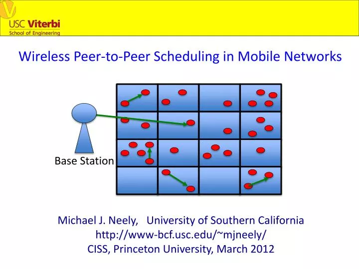
Wireless Peer-to-Peer Scheduling in Mobile Networks. Base Station. Michael J. Neely, University of Southern California http://www- bcf.usc.edu /~ mjneely / CISS, Princeton University, March 2012. Without Device-to-Device Transmission (Example Timeslot). Base Station.

E N D
Wireless Peer-to-Peer Scheduling in Mobile Networks Base Station Michael J. Neely, University of Southern California http://www-bcf.usc.edu/~mjneely/ CISS, Princeton University, March 2012
Without Device-to-Device Transmission (Example Timeslot). Base Station • Want to increase the throughput in wireless systems. • Current system designs cannot support future mobile traffic. • Ideas: • Throughput can be significantly increased by allowing • device-to-device communication. • Exploit file popularity and caching capabilities.
With Device-to-Device Transmission (Example Timeslot). Base Station • Want to increase the throughput in wireless systems. • Current system designs cannot support future mobile traffic. • Ideas: • Throughput can be significantly increased by allowing • device-to-device communication. • Exploit file popularity and caching capabilities.
Example GUI at User Devices • User 2 Modes: • Automatic File Search • Browse a Neighbor • Browse a Social Group • User 2 Public Directory: • Music Videos • Glee Clips • Taylor Swift • YouTube Clips • Clippers Highlights • CISS Talks • User 1 Modes: • Automatic File Search • Browse a Neighbor • Browse a Social Group • User 1 Public Directory: • Music Videos • Lady GaGa • YouTube Clips • Movies • Bob the Builder • Thomas the Train • Neighbors are likely to have Popular Files. • Browsing capabilities induce popularity.
Peer-to-Peer Systems • Much prior work on internet peer-to-peer. • Much prior work on incentives (tokens, tit-for-tat, etc.) • [Neely, GolubchikInfocom 2011] considers utility optimization for general wireless peer-to-peer models, but: • Requires coordination. • Can have large delays in mobile network. • Current paper: • Design for mobile setting with simplified coordination. • Reduce Delays by opportunistically grabbing packets from • current neighbors. • To do this: We will treat a simplified modelwhere each • user only wants 1 “infinitely long” file. • Prove optimality for the simplified model. • Design a heuristic modification for more general systems.
Simple Model: Network Structure N Devices: {Devices} = {Users} U {Access Points} • User devices (example: Handsets) • Want data. • Typically mobile. • Have fewer files cached. • Access point devices (example: Basestations, Femto Nodes) • Don’t want data • Typically non-mobile • Typically have access to many more files.
Simple Model: Transmission Options N Devices: {Devices} = {Users} U {Access Points} • 1-Hop Networking (no relaying). • Access points can transmit to users. • Users can transmit to other users. • Time-Varying Channels, timeslots t in {0, 1, 2, …}. • ω(t) = “topology state” on slot t. • Slot t decision: Choose (μnk(t)) in R(ω(t)). Set of Options for slot t. Transmission matrix • Example sub-cell structure: Decisions are distributed.
Simple Model: File Requests and Availability N Devices: {Devices} = {Users} U {Access Points} • Each user wants 1 file consisting of “infinite” # of packets. • Fk= {Devices that have the file that user k wants}. • Users grab packets of their desired file over time. • xk(t) = ∑aμak(t) = Total user k downloads on slot t. • yk(t) = ∑bμkb(t) = Total user k uploadson slot t.
Stochastic Network Optimization Problem • xk = Time average rate of user k downloads. • yk= Time average rate of user k uploads. Maximize: ∑kφk(xk) Subject to: (1)ακxκ ≤ βκ+ yκfor all users k (2) (μnk(t)) inR(ω(t)) for all t in {0, 1, 2, …} Concave utility functions Tit-for-Tat constraints to incentivize participation
Solution (Lyapunov Optimization) • Virtual queues Hk(t) for tit-for-tat constraints: ακxκ ≤ βκ+ yκ Hk(t) βk+ yk(t) αkxk(t) Hk(t+1) = max[Hk(t) + αkxk(t) – βk – yk(t), 0] • Hk(t) is a reputation queue: • Hk(t) low “good reputation” • Hk(t) high “bad reputation”
Dynamic Algorithm • Maintain a request queueQk(t) and reputation queueHk(t). • User k request decision on slot t: • Maximize: Vφk(γk(t)) – Qk(t)γk(t) • Subject to: 0 ≤ γk(t) ≤ γmax • Transmission Decisions on slot t: • Maximize: ∑ μnk(t)Wnk(t) • Subject to: (μnk(t)) inR(ω(t)) • Update Queues: • Qκ(t+1) = max[Qk(t) + γk(t) – xk(t), 0] • Hk(t+1) = max[Hk(t) + αkxk(t) – βk – yk(t), 0]
What are the weights Wnk(t)? • Transmit decision: Maximize ∑ μnk(t)Wnk(t) • For users n and k: • Wnk(t) = Qk(t) + Hn(t) – αkHk(t) “Differential Reputation” • Like “backpressure” with reputations! • The optimization naturally gives a “token” • mechanism: If your reputation is bad, you • need to improve it to get more downloads!
Performance Theorem • For all sample paths of time-variation • (possibly non-ergodic topology states w(t)), • the queues Qk(t), Hk(t) are deterministically • bounded by O(V). • All tit-for-tat constraints are satisfied. • If w(t) is ergodic, then: • Achieved utility ≥ Optimal utility – O(1/V)
Simulation Scenario Base Station • 1 Base Station, 50 mobile users. • Base station transmission is orthogonal from P2P. • P2P transmissions distributed over sub-cells. • 1 P2P transmission per sub-cell. • Files randomly selected at time 0: • p = Pr[other user has file] = Availability probability
New files chosen at beginning of each phase. Held fixed over 3 phases. • Phase 1: Availiabilityprob = 5% • Phase 2: Availability prob = 10% • Phase 3: Availability prob = 7% • (Even with p = 5%, the P2P traffic is more than twice the BS traffic!)
New files chosen at beginning of each phase. Held fixed over 3 phases. • Phase 1: Availiabilityprob = 5% • Phase 2: Availability prob = 10% • Phase 3: Availability prob = 7% • (This and previous use V=10, a=0.5. Then Q(t) ≤ 12 packets for all t.)
The above shows throughput versus V. • Different tit-for-tat parameters α are shown: • Larger α means more incentives to participate, but optimality is then • more constrained.
The corresponding queue size for the same experiment as previous • slide. • Our analytical bound ensures Queue size ≤ V+2 for all time. • At V=10 (which gives near optimality from previous figure) we get • a queue bound of 12.
Conclusions Base Station • Lyapunov optimization approach to wireless P2P scheduling. • “Backpressure” on Reputations. • P2P leads to significant gains in throughput. • Our algorithm, derived for the simple “infinite file size” assumption, • also works well on finite file sizes and non-ergodic events.