Download
1 / 25
270 likes | 449 Views
Example regulatory control: Distillation. 5 dynamic DOFs (L,V,D,B,VT) Overall objective: Control compositions (x D and x B ) “Obvious” stabilizing loops: Condenser level (M 1 ) Reboiler level (M 2 ) Pressure.

E N D
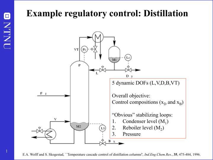
Example regulatory control: Distillation • 5 dynamic DOFs (L,V,D,B,VT) • Overall objective: • Control compositions (xD and xB) • “Obvious” stabilizing loops: • Condenser level (M1) • Reboiler level (M2) • Pressure E.A. Wolff and S. Skogestad, ``Temperature cascade control of distillation columns'', Ind.Eng.Chem.Res., 35, 475-484, 1996.
LV-configuration used for levels (most common) “LV-configuration”: L and V remain as degrees of freedom after level loops are closed Other possibilities: DB, L/D V/B, etc….
Ttop Temperature BUT: To avoid strong sensitivity to disturbances: Temperature profile must also be “stabilized”
Data “column A” • Binary ideal mixture with relative volatility 1.5 • Equimolar feed (zF=0.5) • Both products 99% purity (xD, xB) • 41 stages, feed at stage 20 • Liquid lag: 1.5 min (from top to bottom) • Level control: Tight • Temperature control: Kc=1.84 (1 min closed-loop time constant) • Assume top product (xD) most important → Close loop at top (L) • Composition control (supervisory layer): Decentralized PID • Measurement delay for composition: 6 min
Singular value rule:Tray 27 is most sensitive (6 above feed)
Supervisory control: Primary controlled variables y1 = c = (xD xB)T Regulatory control: Control of y2=T using u2 = L (original DOF) Setpoint y2s = Ts: new DOF for supervisory control Partial control u1 = V
Closed-loop response with decentralized PID-composition control Interactions much smaller with “stabilizing” temperature loop closed … and also disturbance sensitivity is expected smaller
May get improvement with L/D V/B - configuration for level loops Simulations are with decentralized PID-control in supervisory layer Difference smaller if we use multivariable control (MPC)
Conclusion: Stabilizing control distillation • Control problem as seen from layer above becomes much simpler if we control a sensitive temperature inside the column (y2 = T) • Stabilizing control distillation • Condenser level • Reboiler level • Pressure (sometimes left “floating” for optimality) • Column temperature • Most common pairing: • “LV”-configuration for levels • Cooling for pressure • V for T-control (alternatively if top composition most important: L for T-control)
Ls Ts TC Conclusion stabilizing control:Remaining supervisory control problem + may adjust setpoints for p, M1 and M2 (MPC)
Why control temperature at stage 27?Rule: Maximize the scaled gain • Scalar case. Minimum singular value = gain |G| • Maximize scaled gain: |Gs| = |G| / span • |G|: gain from independent variable (u) to candidate controlled variable (c) • span (of c) = variation (of c) = optimal variation in c + control error for c
Assume here that both xD + xB are important • Distillation example • columnn A. u=L. Which temperature to control? • Nominal simulation (gives x0) • One simulation: Gain with constant inputs (u) • Make small change in input (L) • with the other inputs (V) constant • Find gainl = xi/ L • - have also given gains for disturbances (F,z,q) • From process gains: Obtain “optimal” change for candidate measurements to disturbances, • (with input L adjusted to keep both xD and xB close to setpoint, i.e. min ||xD-0.99; xb-0.01|| , with V=constant). • w=[xB,xD]. Then (- Gy pinv(Gw) Gwd + Gyd) d • (Note: Gy=gainl, d=F: Gyd=gainf etc.) • Find xi,opt (yopt) for the following disturbances • F (from 1 to 1.2; has effect!) yoptf • zF from 0.5 to 0.6 yoptz • qF from 1 to 1.2 yoptq • xB from 0.01 to 0.02 yoptxb=0 (no effect) • Control (implementation) error. Assume=0.05 on all stages • Find • scaled-gain = gain/span • where span = abs(yoptf)+abs(yoptz)+abs(yoptq)+0.05 • “Maximize gain rule”: Prefer stage where scaled-gain is large >> res=[x0' gainl' gainf' gainz' gainq'] res = 0.0100 1.0853 0.5862 1.1195 1.0930 0.0143 1.5396 0.8311 1.5893 1.5506 0.0197 2.1134 1.1397 2.1842 2.1285 0.0267 2.8310 1.5247 2.9303 2.8513 0.0355 3.7170 1.9990 3.8539 3.7437 0.0467 4.7929 2.5734 4.9789 4.8273 0.0605 6.0718 3.2542 6.3205 6.1155 0.0776 7.5510 4.0392 7.8779 7.6055 0.0982 9.2028 4.9126 9.6244 9.2694 0.1229 10.9654 5.8404 11.4975 11.0449 0.1515 12.7374 6.7676 13.3931 12.8301 0.1841 14.3808 7.6202 15.1675 14.4857 0.2202 15.7358 8.3133 16.6530 15.8509 0.2587 16.6486 8.7659 17.6861 16.7709 0.2986 17.0057 8.9194 18.1436 17.1311 0.3385 16.7628 8.7524 17.9737 16.8870 0.3770 15.9568 8.2872 17.2098 16.0758 0.4130 14.6955 7.5832 15.9597 14.8058 0.4455 13.1286 6.7215 14.3776 13.2280 0.4742 11.4148 5.7872 12.6286 11.5021 0.4987 9.6930 4.8542 10.8586 9.7680 0.5265 11.0449 5.4538 12.1996 11.1051 0.5578 12.2975 6.0007 13.4225 12.3410 0.5922 13.3469 6.4473 14.4211 13.3727 0.6290 14.0910 6.7478 15.0929 14.0989 0.6675 14.4487 6.8669 15.3588 14.4397 0.7065 14.3766 6.7871 15.1800 14.3528 0.7449 13.8797 6.5135 14.5676 13.8438 0.7816 13.0098 6.0724 13.5807 12.9654 0.8158 11.8545 5.5060 12.3136 11.8051 0.8469 10.5187 4.8635 10.8764 10.4677 0.8744 9.1066 4.1929 9.3765 9.0566 0.8983 7.7071 3.5346 7.9044 7.6602 0.9187 6.3866 2.9184 6.5261 6.3443 0.9358 5.1876 2.3624 5.2829 5.1505 0.9501 4.1314 1.8756 4.1942 4.1000 0.9617 3.2233 1.4592 3.2631 3.1975 0.9712 2.4574 1.1098 2.4816 2.4368 0.9789 1.8211 0.8208 1.8355 1.8053 0.9851 1.2990 0.5848 1.3077 1.2875 0.9900 0.8747 0.3938 0.8805 0.8670
Assume here that both xD + xB are important u=L >> [yoptf yoptq yoptz span] ans = 0.0077 0.0014 0.0011 0.0601 0.0108 0.0019 0.0016 0.0644 0.0146 0.0027 0.0025 0.0698 0.0192 0.0036 0.0038 0.0765 0.0246 0.0047 0.0056 0.0849 0.0309 0.0061 0.0082 0.0951 0.0379 0.0077 0.0117 0.1073 0.0456 0.0096 0.0163 0.1215 0.0536 0.0118 0.0222 0.1375 0.0612 0.0141 0.0294 0.1546 0.0678 0.0164 0.0379 0.1720 0.0724 0.0186 0.0474 0.1884 0.0742 0.0204 0.0575 0.2022 0.0726 0.0217 0.0676 0.2119 0.0673 0.0222 0.0769 0.2164 0.0584 0.0220 0.0847 0.2151 0.0467 0.0211 0.0906 0.2085 0.0332 0.0196 0.0945 0.1973 0.0190 0.0177 0.0964 0.1831 0.0052 0.0155 0.0966 0.1673 -0.0076 0.0134 0.0955 0.1665 -0.0242 0.0102 0.0915 0.1758 -0.0412 0.0066 0.0858 0.1837 -0.0578 0.0029 0.0784 0.1892 -0.0728 -0.0008 0.0696 0.1932 -0.0851 -0.0042 0.0596 0.1990 -0.0938 -0.0072 0.0491 0.2001 -0.0984 -0.0095 0.0387 0.1965 -0.0988 -0.0111 0.0288 0.1887 -0.0954 -0.0119 0.0202 0.1775 -0.0891 -0.0120 0.0129 0.1640 -0.0807 -0.0115 0.0072 0.1494 -0.0711 -0.0107 0.0030 0.1347 -0.0610 -0.0095 0.0001 0.1206 -0.0512 -0.0083 -0.0017 0.1112 -0.0419 -0.0070 -0.0027 0.1016 -0.0335 -0.0057 -0.0030 0.0923 -0.0261 -0.0045 -0.0029 0.0835 -0.0197 -0.0035 -0.0025 0.0756 -0.0142 -0.0025 -0.0020 0.0686 -0.0095 -0.0017 -0.0013 0.0626 >> Gw Gw = 1.0853 0.8747 Gwf = 0.5862 0.3938 >> yoptf = (-gain'*pinv(Gw)*Gwf + gainf')*0.2 >> yoptq = (-gain'*pinv(Gw)*Gwq + gainq')*0.2 >> yoptz = (-gain'*pinv(Gw)*Gwz + gainz')*0.1 have checked with nonlinear simulation. OK!
Assume here that both xD + xB are important u=L: max. on stage 15 (below feed stage) In practice (because of dynamics): Will use tray in top (peak at 27) >> span = abs(yoptf)+abs(yoptz)+abs(yoptq)+0.05; >> plot(gainl’./span)
Assume here that both xD + xB are important >> [yoptf yoptq yoptz span] ans = 0.0065 -0.0008 -0.0000 0.0573 0.0091 -0.0011 0.0001 0.0603 0.0123 -0.0014 0.0004 0.0641 0.0162 -0.0018 0.0010 0.0690 0.0208 -0.0022 0.0021 0.0750 0.0260 -0.0025 0.0038 0.0823 0.0320 -0.0029 0.0062 0.0911 0.0384 -0.0032 0.0097 0.1013 0.0450 -0.0033 0.0144 0.1128 0.0513 -0.0033 0.0205 0.1251 0.0567 -0.0030 0.0280 0.1377 0.0604 -0.0023 0.0367 0.1495 0.0617 -0.0013 0.0464 0.1594 0.0601 0.0001 0.0565 0.1667 0.0553 0.0019 0.0664 0.1736 0.0476 0.0040 0.0754 0.1770 0.0376 0.0063 0.0830 0.1769 0.0262 0.0086 0.0888 0.1736 0.0143 0.0109 0.0929 0.1681 0.0028 0.0130 0.0952 0.1609 -0.0078 0.0148 0.0962 0.1688 -0.0221 0.0165 0.0946 0.1832 -0.0367 0.0180 0.0915 0.1962 -0.0510 0.0191 0.0866 0.2067 -0.0639 0.0197 0.0800 0.2136 -0.0744 0.0198 0.0718 0.2160 -0.0819 0.0192 0.0625 0.2137 -0.0858 0.0182 0.0527 0.2067 -0.0860 0.0167 0.0430 0.1957 -0.0831 0.0149 0.0338 0.1818 -0.0775 0.0130 0.0256 0.1662 -0.0702 0.0111 0.0187 0.1500 -0.0618 0.0093 0.0131 0.1341 -0.0530 0.0076 0.0088 0.1194 -0.0444 0.0061 0.0056 0.1061 -0.0364 0.0048 0.0033 0.0945 -0.0291 0.0037 0.0018 0.0846 -0.0226 0.0028 0.0008 0.0763 -0.0170 0.0021 0.0003 0.0694 -0.0123 0.0015 0.0001 0.0638 -0.0083 0.0010 0.0000 0.0593 u=V Gwv = -1.0975 -0.8625 Gwf = 0.5862 0.3938 >> yoptf = (-gainv'*pinv(Gwv)*Gwf + gainf')*0.2 >> yoptq = (-gainv'*pinv(Gwv)*Gwq + gainq')*0.2 >> yoptz = (-gainv'*pinv(Gwv)*Gwz + gainz')*0.1 >> span = abs(yoptf)+abs(yoptz)+abs(yoptq)+0.05; >> plot(gainv'./span)
Assume here that both xD + xB are important u=V: sharp max. on stage 14 (below feed stage) >> span = abs(yoptf)+abs(yoptz)+abs(yoptq)+0.05; >> plot(gain’./span)
COMMENT! NEED to be careful about nonlinearity! Effect of step size in V: delta=0.005 Gw = -0.7600 -1.1956 delta=0.001 Gw = -1.0276 -0.9326 delta=0.0002 Gw = -1.0843 -0.8758 delta=0.00005 Gw = -1.0948 -0.8653 delta=0.00001 Gw = -1.0975 -0.8625