Download

1 / 35
390 likes | 769 Views
ECON 100 Tutorial: Week 20. www.lancaster.ac.uk/postgrad/murphys4/ s.murphy5@lancaster.ac.uk office: LUMS C85. Some notes for the last section of ECON 100.

E N D
ECON 100 Tutorial: Week 20 www.lancaster.ac.uk/postgrad/murphys4/ s.murphy5@lancaster.ac.uk office: LUMS C85
Some notes for the last section of ECON 100 • You’ve had some experience with David Peele’s questions – on Exam 4, I expect to see similar style of questions from him, so practice the maths that he is teaching. • Gerry Steele doesn’t change his questions much from year to year – so past exams are a great resource for preparing for Exam 4. (Past papers can be found on the student registry site; select a year, select ECON 100, then look at approximately the last 10 questions on each year’s exam.) • Gerry’s Tutorial Questions are also great for preparing for Exam 4.
Question 1 What precisely did A.W. Phillips show on the vertical axis in his original presentation of the ‘Phillips curve’? (http://www.jstor.org/stable/2550759) ‘Rate of change of money wage rates, % per year’ Note: Some texts show inflation on the Y axis when drawing the Phillips Curve. Gerry prefers to use this notation instead. Question 2 looks at why he makes this choice.
Question 2 How was ‘inflation’ irrelevant to the original presentation of the ‘Phillips curve’? ‘Inflation’ was not the general experience of the UK economy during the period of Phillip’s analysis (1861-1957). Rather, for much of the 1920s and 1930s, prices were falling’ ’
Question 3 The Phillips inflation-unemployment relationship is better described as “L-shaped” rather than a curve. Explain. ΔW/W Phillips’s explanation: ‘When the demand for labour is high we should expect employers to bid wage rates up quite rapidly. On the other hand it appears that workers are reluctant to offer their services at less than prevailing rates when the demand for labour is low’ (Gerry covers this in lecture 1) % unemployment rate
Question 4 – Gerry’s solution In the 1960s, ‘the Keynes-Phillips orthodoxy was sailing on smooth waters, the object of much congratulation, rather like the liner Titanic prior to its collision with the fateful iceberg’ (Edmund Phelps). What is the nature of ‘the Keynes-Phillips orthodoxy’ and why was a collision inevitable? Steele’s suggested solution: The Keynes-Phillips orthodoxy argues that inflation cannot occur with large-scale unemployment: ‘ … an increase in the quantity of money will have no effect whatever on prices, so long as there is any unemployment …’ (TGT: 295) ‘ … the general level of prices will not rise very much as output increases, so long as there are available efficient unemployed resources of every type.’ (TGT: 300) As subsequent analysis (the Friedman-Phelps expectations-augmented Phillips curve) predicts, the co-existence of high inflation and high unemployed is likely when monetary growth is excessive (i.e., when ΔMS/MS > ΔMD/MD, demand-pull inflation is results)
Question 4 – another look What is the nature of ‘the Keynes-Phillips orthodoxy’ and why was a collision inevitable? Keynes-Phillips say that if you grow money supply (MS), you won’t have inflation if, at the same time, you have unemployment. Steele’s approach tells us: The “inevitable collision” that Friedman-Phelps (expectations-augmented Phillips curve) predicted is that: If Monetary growth is excessive (i.e., ΔMS/MS > ΔMD/MD), then high inflation and high unemployment can actually occur at the same time (i.e., Gerry calls it demand-pull inflation) Usually (not Gerry’s method) cost-push and demand-pull inflation are presented using AS/AD. • The graph on the right shows the Phillips Curve over time. (using US data) • In the late 1960’s, we are on SPRC0, and it looks like Phillips’ assessment is correct. • By the late 1970’s and early ‘80’s, we see both high unemployment and high inflation (SRPC3). In this example, this came about because high import prices (particularly oil), rather than because of excessive monetary growth, which is what Friedman-Phelps were talking about.
Cost-push inflation vs. Demand-pull inflation 1973: Price of oil ↑ OPEC oil embargo. 1979: Price of oil ↑ Iranian revolution. Oil is a major factor of production, so if P ↑ and consumption ↓then production ↓, pushing aggregate supply leftward. This led to what is known as stagflation. What kind of inflation is this? The high inflation in the late 1970s is an example of cost-push inflation. Late 1960’s: G↑ due to the Vietnam war 1965: G↑ due to US’ War on Poverty. Insufficient increases in taxation led to deficit spending and a rightward shift in the aggregate demand curve. What kind of inflation is this? The high inflation in the late 1960s relative to the early 1960s is an example of demand-pull inflation.
Cost-push inflation vs. Demand-pull inflation 1973: Price of oil ↑ OPEC oil embargo. 1979: Price of oil ↑ Iranian revolution. Oil is a major factor of production, so if P ↑ and consumption ↓then production ↓, pushing aggregate supply leftward. Steele presents the idea that cost-push inflation we’ve been describing is actually price-inflation, not monetary inflation. Some economists do not think that price-inflation should be included in the definition of inflation. Late 1960’s: G↑ due to the Vietnam war 1965: G↑ due to US’ War on Poverty. Insufficient increases in taxation led to deficit spending and a rightward shift in the aggregate demand curve. Steele notes that the late 1960’s and early 1970’s coincided with the end of the fixed exchange rate and the beginning of new expansionist policies in the central bank of England. He thinks that this demand-pull inflation continued to drive inflation in the 1970s. Note: To properly understand Gerry’s materials, the best thing to do is review the lectures and lecture slides as well as any reading material he puts up on Moodle.
Question 5(a) With the expectations-augmented Phillips curve represented conventionally as ΔW/W = f(U) + φ(ΔP/P)e Identify each of the variables: ΔW/W proportionate increase in wages P prices U percentage unemployment rate (ΔP/P)e expected proportionate increase in prices
Question 5(b) With the expectations-augmented Phillips curve represented conventionally as ΔW/W = f(U) + φ(ΔP/P)e What sign respectively would be expected for the coefficients f and φ. Explain. f negative. There is an inverse relationship between unemployment and Δmoney wages. This is the same as in the original Phillips curve. φ positive When workers accept employment contracts, they choose wages that reflect anticipated price changes. This is expectations-augmented part.
Question 5(c) With the expectations-augmented Phillips curve represented conventionally as ΔW/W = f(U) + φ(ΔP/P)e Which description is usually given for φ < 1. Explain. money illusion If the rate of increase in wages < the rate of increase in prices, then, workers are being paid less in real terms. The workers would be mistaken to accept this, but they might due to money illusion. Money illusion is the idea that if you’re paid more you must be wealthier. You’re only wealthier if you’re paid more relative to the price levels.
Question 5(d) With the expectations-augmented Phillips curve represented conventionally as ΔW/W = f(U) + φ(ΔP/P)e What is the ‘reservation wage’ in the analysis of job search? the minimum level of acceptable wage offer
Question 5(e) With the expectations-augmented Phillips curve represented conventionally as ΔW/W = f(U) + φ(ΔP/P)e What is the likely impact upon the reservation wage as the duration of unemployment increases? reservation wage falls
Question 5(f) With the expectations-augmented Phillips curve represented conventionally as ΔW/W = f(U) + φ(ΔP/P)e What is the likely impact upon unemployment if unemployment benefits increase? unemployment is likely to rise as job search is extended
Question 5(g) With the expectations-augmented Phillips curve represented conventionally as ΔW/W = f(U) + φ(ΔP/P)e Explain the likely impact upon unemployment of (ΔP/P) > (ΔP/P)e. So, we are asking, if the proportionate change in prices is greater than the expected proportionate change in prices, what will be the impact on unemployment. (Note, this is another way of saying if inflation > expected inflation, or if we underestimate the inflation rate) The period of job search is likely to be curtailed (cut short), if the inflation rate is underestimated.
Question 5(h) With the expectations-augmented Phillips curve represented conventionally as ΔW/W = f(U) + φ(ΔP/P)e Explain the likely impact upon unemployment of (ΔP/P) = (ΔP/P)e. unemployment finds its ‘natural rate’
Question 6 With prices rising at 4.0 percent annually, and wages rising at 3.5 percent per annually, what would be the percentage reduction in real wages over a five year period? To answer this question, we need to the difference between future real wages and the current period real wages. To find the future period real wages, we have to calculate three things here: real wages, and wages in a future period, and prices in a future period. Here are the three equations we’ll need: Real Wages = nominal wage ÷ prices Wagefuture period = Wagecurrent period * (1 + growth ratewages)ΔT Pricefuture period = Pricecurrent period * (1 + growth rateprices)ΔT We can put it all together into the following equation: Real Wagesfutureperiod= Wagecurrent period*(1 + growth ratewages)ΔT ÷ Pricecurrent period*(1 + growth rateprices)ΔT
Question 6 ctd. With prices rising at 4.0 percent annually, and earnings rising at 3.5 percent per annually, what would be the percentage reduction in real wages over a five year period? First, find Real Wages (R) in Year 5: R5 = = = Next, find the percentage change from Year 1 to 5: Percentage Change = 1 - = 1 - = 2.4%
The Phillips Curve The following game is a fun way to look at the relationship between unemployment and inflation (the Phillips Curve). It allows you to pretend that you are the Central Bank and can set interest rates as a tool to control inflation and unemployment. A high interest rate will attract people to purchasing bonds and holding less money, restricting money supply and reducing inflation. A low interest rate will make investments more attractive. People will invest in capital stock with a rate of return greater than the return on bonds. Because the return on bonds is low, this implies lots of capital investments will seem profitable. These investments will create jobs and lower unemployment. In summary: IR↑ → inflation↓ IR↓ → unemployment↓
The game lasts 16 rounds (16 quarters = 4 years). The overall goal is to keep the economy in good shape so that you get re-elected. Remember: IR↑ → inflation↓ IR↓ → unemployment↓ Inflation and unemployment don’t respond immediately, there are some lags, so it’s good to start by slightly raising the interest rate. We’ll divide the class into two groups: Each round, both groups discuss their choices and the President makes a recommendation to the Fed. The Fed has a few second to discuss and the Chairman makes the final decision. It’s not as easy as it sounds – let’s see how well you do: http://sffed-education.org/chairman/ Executive BranchFederal Reserve Bank Choose a: President Chairman Goal: keep unemployment low keep inflation at/slightly below near 5% the target rate: 2%
Next Week Check Moodle for a tutorial worksheet and work through it before coming to class. I’ll try to add in some examples of past exam multiple choice questions that relate to the tutorial, if possible. Note: Tuesday’s Tutorial will move to 1:00 PM in County Main SR 2 for the remainder of the term. If you have a timetable problem, contact Sarah Ross.
Examples of Past Exam Multiple Choice Questions that relate to this week’s tutorial
The original Phillips curve identified a robust correlation between: (a) unemployment and the rate of change of real wage rates (b) unemployment and the rate of change of money wage rates (c) wage levels and unemployment (d) wage levels and inflation 2012 Exam Q35
Phillips Curve • Inflation is a change in money wages
The hypothesis of the expectations-augmented Phillips curve holds that: • employment contracts fully accommodate the rate of price inflation • job-seekers never make systematic errors • wage settlements are partially determined by the expected rate of price inflation • reservation wages are determined by minimum wage legislation 2010 Exam Q32
Expectations Augmented Phillips Curve Initially, unemployment and inflation are at point A. Expansionist monetary policy would increase consumption, shifting to point B along the Phillips curve Unemployment is reduced but there is a trade off; inflation. After a short period, agents will associate expansionist policies with inflation and will push for higher wages. This will stop the consumption stimulus and also de-incentivize hiring. Agents will shift their expectations curves to point C.
According to Friedman’s re-interpretation of the Phillips Curve, if inflationary expectations rise, the Phillips curve: a) shifts down b) shifts up c) becomes flatter d) becomes steeper 2011 Exam Q32
Expectations Augmented Phillips Curve Initially, unemployment and inflation are at point A. Expansionist monetary policy would increase consumption, shifting to point B along the Phillips curve Unemployment is reduced but there is a trade off; inflation. After a short period, agents will associate expansionist policies with inflation and will push for higher wages. This will stop the consumption stimulus and also de-incentivize hiring. Agents will shift their expectations curves to point C.
If job seekers under-estimate the rate of inflation, the duration of the job-search: (a) shortens, so that unemployment tends to rise (b) lengthens, so that unemployment tends to fall (c) shortens, so that unemployment tends to fall (d) lengthens, so that unemployment tends to rise 2012 Exam Q36
If job seekers under-estimate the rate of inflation: (DP/P) >(DP/P)e • Then they will over-estimate the value of an offered wage contract • And will accept a lower real wage more readily • And thus will have a shorter period of unemployment • And unemployment will fall below the natural rate, U<Un If the causation is reversed, when actual inflation is below the expected rate of inflation, (DP/P) <(DP/P)ethen unemployment will be above the natural rate: U>Un
Identify the missing word(s): Goodhart’s Law states ‘that any ____I____ will tend to collapse once pressure is placed upon it for control purposes.’ • monetary target • observed statistical regularity • fiscal budgetary stance • structured investment 2010 Exam Q35
Goodhart’s Law “Any observed statistical regularity will tend to collapse once pressure is placed upon it for control purposes.” … an expansion of aggregate demand was expected to (increase inflation and to) lower unemployment … but when the authorities attempted to achieve this, the inflation -unemployment regularity collapsed …
Suppose that national income (measured in 1990 prices) is £1000 billion. Suppose further that prices have doubled since 1990 and that the typical unit of money circulates around the economy 20 times per year. What is the money supply? • £50 billion • £100 billion • £150 billion • £200 billion 2010 Exam Q36
MV = QP We know that: V = 20 Q = 1000 P = 2 So, solving for M: MV=PQ M = QP/V M = 1000*2/20 M = 100