Download
1 / 29
290 likes | 382 Views
Future 2 Soft Constraints Transfer Limit Hardening. By the NEEM-TX Subteam SSC Meeting June 6, 2011. Process of Applying Transfer Limit Hardening (TLH) Methodology.

E N D
Future 2 Soft ConstraintsTransfer Limit Hardening By the NEEM-TX Subteam SSC Meeting June 6, 2011
Process of Applying Transfer Limit Hardening (TLH) Methodology • For each future, SSC will decide whether to use Baseline Infrastructure transfer limits or transfer limits based on the soft constraint sensitivity results • NEEM soft constraint results will be assessed with the transfer hardening method selected today for Futures 2, 3, 5, 6, 7, and 8 • The approved transfer limit hardening methodology will be applied to the preferred soft constraint sensitivity flows (i.e., OL75 or OL25 where applicable) to develop new fixed transfer limits that will be used for the remaining sensitivities of that future 2
Goals of Presentation • Future 2 Soft Constraint Sensitivities 1 & 2 (OL75/OL25) • TLH Methodology Options • RHC Revisions • Parameter Adjustments • Anomaly Treatment Considerations
TLH Transfer Limit Decision Item 2 • Option 1: OL75 • Option 2: OL25
Generation Build Comparison • OL25 Super-region Cumulative Capacity build minus OL75 Super-region Cumulative Capacity build • Wind resources move from PJM and MISO to southwest • Northeast wind resources displaced by HQ pseudo-generator • Some increase in Southwest wind likely displacing South nuclear and CC
Option 1: OL75 • Certain stakeholder believe OL75 is likely to be a more “cost-effective” transmission expansion • OL75 and OL25 produce similar level of aggregate generation build • OL25 builds 3 GW more wind, but produces 7% more wind energy (+65,331,000 MWh) • OL25 shifts wind generation to windier areas • Certain stakeholders believe OL25 flows overly concentrate generation in a single region (MISO_W) producing unrealistic results • i.e. OL25 creates more anomalies
Option 2: OL25 • Certain stakeholders believe OL25 increases transmission build to a level more appropriate for a nationally-focused future • Certain stakeholders believe that without the greater increase in inter-super-region transfer limits produced by OL25, national and regional futures are unlikely to produce meaningful differences that we can learn from • Certain stakeholders believe using OL25 will create a more appropriate “book-end” for the study purposes
Cost Savings Considerations • Relative to base run, increased transfer limits may reduce generation and emissions costs for eastern interconnection • Cost savings could be used to evaluate some economic benefits from transfer limit expansions • A comparison of cost savings, expressed in present value, from the OL75 and OL25 runs may help inform the transfer limit decision • Certain stakeholders believe that cost savings information should be used only for information and not as a deciding criteria between OL75 and OL25
Comparison of Cost Savings • Savings represent reductions in CRA’s “Total Cost” results for all NEEM regions in the Eastern Interconnection combined. See accompanying fact sheet for more explanation on the metric. • Transfer limit expansions represent the sum of all suggested new capacity averaged across the three Transfer Limit Hardening (TLH) methods under both default and relaxed parameter values. • Savings / MW are the quotient of reductions in “Total Cost” and expansions.
Overview of theTLH Methodology Options • Three proposed methodologies • Ruthven/Hadley/Chattopadhyay (RHC) • Focused on pipe capacity factors and shadow prices • Methodology revised from original specifications • NGO • Focused on Flow Duration Curve and fraction of time the pipe is full • Johnson • Focused on total energy flow and base line utilization • All methodologies based on 2020-35 data 10
Maritimes 12 HQ OH MAPP CA 8 NEISO 9 NWPP 4 14 MISO WUMS NYISO A-F 10 MAPP US MISO W 2 1 6 MISO MI NYISO GHI 5 13 RMPA MISO IN NE MISO MO IL NYISO J & K Non RTO Midwest 3 SPP N 11 BAU OL25 PJM Rest of MAAC PJM Eastern MAAC PJM Rest of RTO ENTERGY 5 TVA VACA SPP S AZ NM SNV SOCO ERCOT 11 FRCC
Maritimes HQ OH MAPP CA NEISO 11 17 15 NWPP MISO WUMS 14 NYISO A-F MAPP US MISO W 16 19 MISO MI 8 1 4 NYISO GHI 9 6 12 RMPA 10 MISO IN NE MISO MO IL NYISO J & K Non RTO Midwest 18 3 13 SPP N 2 F2 OL75 PJM Rest of MAAC PJM Eastern MAAC PJM Rest of RTO 20 ENTERGY TVA 7 VACA SPP S AZ NM SNV 5 SOCO ERCOT 12 FRCC
Maritimes HQ OH MAPP CA NEISO 20 19 13 NWPP MISO WUMS NYISO A-F MAPP US MISO W 2 6 14 MISO MI 1 15 NYISO GHI 8 5 4 RMPA 11 MISO IN NE MISO MO IL NYISO J & K Non RTO Midwest 12 18 7 SPP N F2 OL25 3 PJM Rest of MAAC PJM Eastern MAAC PJM Rest of RTO 17 16 ENTERGY TVA 9 VACA SPP S AZ NM SNV 10 SOCO ERCOT 13 FRCC
RHC Revisions • Original RHC specifications yielded desired pipe capacity factors designers thought were inappropriate • Max/Min Desired Capacity Factors Installed • 85% - 40% for total flow • 35% - 15% for overload flow • Prevents extremely low desired capacity factors seen with old RCH • Propose: Linear Curve based on relative shadow price • CF=(x-Shadow Price)/x; x=75% of the max future base case shadow price • Curve will self-adjust for each future relative to shadow prices • Tested on F1, RHC New yields similar results to RHC Old
Alternative THL Methodologies Top 10 InterfacesTransfer Limits (MW)
Future 2 Sensitivity 1 - OL75 Alternative THL Methodologies with Default Parameters 19
Future 2 Sensitivity 2 – OL25 Alternative THL Methodologies with Default Parameters 20
Parameter Adjustments • Each methodology contains adjustable input parameters • Default parameters based on developer understanding of what is “reasonable” but are arbitrary • Default parameters are not derived from actual transmission planning processes • Relaxed – Parameters adjusted downward 10% points (e.g. RHC max capacity factor decreased from 85% to 75%) • Constrained – Parameters adjusted upward by 10% points (e.g. RHC max capacity factor increased from 85% to 95%)
Future 2 Sensitivity 1 - OL75 Average of THL Methodologies with Adjusted Parameters 22
Future 2 Sensitivity 2 – OL25 Average of THL Methodologies with Adjusted Parameters 23
Adjusted Parameters’Aggregate Transfer Limit Increase (MW) Using Average of THL Methodologies 24
TLH Transfer Limit Decision Item 1 Subteam has consensus in supporting the average of the three methodologies but not consensus around appropriate parameters • Option 1 • Use default parameters • Option 2 • Use relaxed parameters
Option Parameters Option 1 Parameters Option 2 Parameters RHC Total Flow Min/Max CF: 30%-75% OL Flow Min/Max CF: 5%-25% Johnson Utilization Threshold: 80% Average CF: 65% NGO Flow Duration Curve Threshold: 10% • RHC • Total Flow Min/Max CF: 40%-85% • OL Flow Min/Max CF: 15%-35% • Johnson • Utilization Threshold: 90% • Average CF: 75% • NGO • Flow Duration Curve Threshold: 20%
Anomaly Treatment Considerations • Make no adjustments for anomalies • “Reality” check on large transfer limit expansions will be applied when SSC decides on Phase II build-outs • “Reality” check will require use of a sensitivity • OL25 more likely to need more adjustments for anomalous results than OL75 • Some anomalies will likely persist throughout all futures • e.g. MISO will always direct as much gas build as possible to MISO_WUMS • Changes for anomalies could lead to lower high-level transmission cost estimate