Download
1 / 32
430 likes | 770 Views
Chapter 4. Discrete Probability Distributions. Probability Distributions. § 4.1. x. x. 0. 0. 2. 2. 4. 4. 6. 6. 8. 8. 10. 10. Random Variables. A random variable x represents a numerical value associated with each outcome of a probability distribution.

E N D
Chapter 4 Discrete Probability Distributions
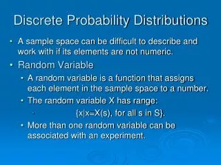
x x 0 0 2 2 4 4 6 6 8 8 10 10 Random Variables A random variable xrepresents a numerical value associated with each outcome of a probability distribution. A random variable is discrete if it has a finite or countable number of possible outcomes that can be listed. A random variable is continuous if it has an uncountable number or possible outcomes, represented by the intervals on a number line.
Random Variables Example: Decide if the random variable x is discrete or continuous. a.) The distance your car travels on a tank of gas The distance your car travels is a continuous random variable because it is a measurement that cannot be counted. (All measurements are continuous random variables.) b.) The number of students in a statistics class The number of students is a discrete random variable because it can be counted.
Discrete Probability Distributions A discrete probability distribution lists each possible value the random variable can assume, together with its probability. A probability distribution must satisfy the following conditions. In Words In Symbols 1. The probability of each value of the discrete random variable is between 0 and 1, inclusive. 0 P (x) 1 2. The sum of all the probabilities is 1. ΣP (x) = 1
Constructing a Discrete Probability Distribution Guidelines Let x be a discrete random variable with possible outcomes x1, x2, … , xn. 1. Make a frequency distribution for the possible outcomes. 2. Find the sum of the frequencies. 3. Find the probability of each possible outcome by dividing its frequency by the sum of the frequencies. 4. Check that each probability is between 0 and 1 and that the sum is 1.
1 2 Each probability is between 0 and 1. The sum of the probabilities is 1. Constructing a Discrete Probability Distribution Example: The spinner below is divided into two sections. The probability of landing on the 1 is 0.25. The probability of landing on the 2 is 0.75. Let x be the number the spinner lands on. Construct a probability distribution for the random variable x.
1 2 Spin a 1 on the first spin. “and” Spin a 1 on the second spin. Constructing a Discrete Probability Distribution Example: The spinner below is spun two times. The probability of landing on the 1 is 0.25. The probability of landing on the 2 is 0.75. Let x be the sum of the two spins. Construct a probability distribution for the random variable x. The possible sums are 2, 3, and 4. P (sum of 2) = 0.25 0.25 = 0.0625 Continued.
1 2 Spin a 1 on the first spin. Spin a 2 on the first spin. “and” “and” Spin a 2 on the second spin. Spin a 1 on the second spin. 0.1875 + 0.1875 Constructing a Discrete Probability Distribution Example continued: P (sum of 3) = 0.25 0.75 = 0.1875 “or” P (sum of 3) = 0.75 0.25 = 0.1875 0.375 Continued.
1 2 Spin a 2 on the first spin. “and” Spin a 2 on the second spin. Constructing a Discrete Probability Distribution Example continued: P (sum of 4) = 0.75 0.75 = 0.5625 Each probability is between 0 and 1, and the sum of the probabilities is 1. 0.5625
P(x) Sum of Two Spins 0.6 Probability 0.5 0.4 0.3 0.2 x 0 0.1 2 3 4 Sum Graphing a Discrete Probability Distribution Example: Graph the following probability distribution using a histogram.
Mean The mean of a discrete random variable is given by μ = ΣxP(x). Each value of x is multiplied by its corresponding probability and the products are added. Example: Find the mean of the probability distribution for the sum of the two spins. ΣxP(x) = 3.5 The mean for the two spins is 3.5.
Variance The variance of a discrete random variable is given by 2 = Σ(x – μ)2P (x). Example: Find the variance of the probability distribution for the sum of the two spins. The mean is 3.5. ΣP(x)(x – 2)2 0.376 The variance for the two spins is approximately 0.376
Standard Deviation The standarddeviation of a discrete random variable is given by Example: Find the standard deviation of the probability distribution for the sum of the two spins. The variance is 0.376. Most of the sums differ from the mean by no more than 0.6 points.
Expected Value The expected value of a discrete random variable is equal to the mean of the random variable. Expected Value = E(x) = μ=ΣxP(x). Example: At a raffle, 500 tickets are sold for $1 each for two prizes of $100 and $50. What is the expected value of your gain? Your gain for the $100 prize is $100 – $1 = $99. Your gain for the $50 prize is $50 – $1 = $49. Write a probability distribution for the possible gains (or outcomes). Continued.
Winning no prize Expected Value Example continued: At a raffle, 500 tickets are sold for $1 each for two prizes of $100 and $50. What is the expected value of your gain? E(x) =ΣxP(x). $99 $49 –$2 Because the expected value is negative, you can expect to lose $0.70 for each ticket you buy.
Binomial Distributions § 4.2
Binomial Experiments A binomial experiment is a probability experiment that satisfies the following conditions. 1. The experiment is repeated for a fixed number of trials, where each trial is independent of other trials. 2. There are only two possible outcomes of interest for each trial. The outcomes can be classified as a success (S) or as a failure (F). 3. The probability of a success P (S) is the same for each trial. 4. The random variable x counts the number of successful trials.
Notation for Binomial Experiments Symbol Description n The number of times a trial is repeated. p = P (S) The probability of success in a single trial. q = P (F) The probability of failure in a single trial. (q = 1 – p) x The random variable represents a count of the number of successes in n trials: x = 0, 1, 2, 3, … , n.
Binomial Experiments Example: Decide whether the experiment is a binomial experiment. If it is, specify the values of n, p, and q, and list the possible values of the random variable x. If it is not a binomial experiment, explain why. • You randomly select a card from a deck of cards, and note if the card is an Ace. You then put the card back and repeat this process 8 times. This is a binomial experiment. Each of the 8 selections represent an independent trial because the card is replaced before the next one is drawn. There are only two possible outcomes: either the card is an Ace or not.
Binomial Experiments Example: Decide whether the experiment is a binomial experiment. If it is, specify the values of n, p, and q, and list the possible values of the random variable x. If it is not a binomial experiment, explain why. • You roll a die 10 times and note the number the die lands on. This is not a binomial experiment. While each trial (roll) is independent, there are more than two possible outcomes: 1, 2, 3, 4, 5, and 6.
p = the probability of selecting a red chip Binomial Probability Formula In a binomial experiment, the probability of exactly x successes in n trials is Example: A bag contains 10 chips. 3 of the chips are red, 5 of the chips are white, and 2 of the chips are blue. Three chips are selected, with replacement. Find the probability that you select exactly one red chip. q = 1 – p = 0.7 n = 3 x = 1
The binomial probability formula is used to find each probability. p = the probability of selecting a red chip Binomial Probability Distribution Example: A bag contains 10 chips. 3 of the chips are red, 5 of the chips are white, and 2 of the chips are blue. Four chips are selected, with replacement. Create a probability distribution for the number of red chips selected. q = 1 – p = 0.7 n = 4 x = 0, 1, 2, 3, 4
Complement Finding Probabilities Example: The following probability distribution represents the probability of selecting 0, 1, 2, 3, or 4 red chips when 4 chips are selected. a.) Find the probability of selecting no more than 3 red chips. b.) Find the probability of selecting at least 1 red chip. a.) P (no more than 3) = P (x 3) = P (0) + P (1) + P (2) + P (3) = 0.24 + 0.412 + 0.265 + 0.076 = 0.993 b.) P (at least 1) = P (x 1) = 1 – P (0) = 1 – 0.24 = 0.76
P (x) Selecting Red Chips 0.5 Probability 0.4 0.3 0.2 x 0 0.1 Number of red chips 0 2 1 3 4 Graphing Binomial Probabilities Example: The following probability distribution represents the probability of selecting 0, 1, 2, 3, or 4 red chips when 4 chips are selected. Graph the distribution using a histogram.
Mean, Variance and Standard Deviation Population Parameters of a Binomial Distribution Mean: Variance: Standard deviation: Example: One out of 5 students at a local college say that they skip breakfast in the morning. Find the mean, variance and standard deviation if 10 students are randomly selected.
Geometric Distribution A geometric distribution is a discrete probability distribution of a random variable x that satisfies the following conditions. 1. A trial is repeated until a success occurs. 2. The repeated trials are independent of each other. 3. The probability of a success p is constant for each trial. The probability that the first success will occur on trial xis P (x) = p(q)x – 1, where q = 1 – p.
Geometric Distribution Example: A fast food chain puts a winning game piece on every fifth package of French fries. Find the probability that you will win a prize, a.) with your third purchase of French fries, b.) with your third or fourth purchase of French fries. p = 0.20 q = 0.80 a.)x = 3 b.)x = 3, 4 P (3) = (0.2)(0.8)3 – 1 P (3 or 4) = P (3) + P (4) = (0.2)(0.8)2 0.128 + 0.102 = (0.2)(0.64) 0.230 = 0.128
Geometric Distribution Example: A fast food chain puts a winning game piece on every fifth package of French fries. Find the probability that you will win a prize, a.) with your third purchase of French fries, b.) with your third or fourth purchase of French fries. p = 0.20 q = 0.80 a.)x = 3 b.)x = 3, 4 P (3) = (0.2)(0.8)3 – 1 P (3 or 4) = P (3) + P (4) = (0.2)(0.8)2 0.128 + 0.102 = (0.2)(0.64) 0.230 = 0.128
Poisson Distribution The Poisson distribution is a discrete probability distribution of a random variable x that satisfies the following conditions. 1. The experiment consists of counting the number of times an event, x, occurs in a given interval. The interval can be an interval of time, area, or volume. 2. The probability of the event occurring is the same for each interval. 3. The number of occurrences in one interval is independent of the number of occurrences in other intervals. The probability of exactly x occurrences in an interval is where e 2.71818 and μis the mean number of occurrences.
Poisson Distribution Example: The mean number of power outages in the city of Brunswick is 4 per year. Find the probability that in a given year, a.) there are exactly 3 outages, b.) there are more than 3 outages.