It follows that

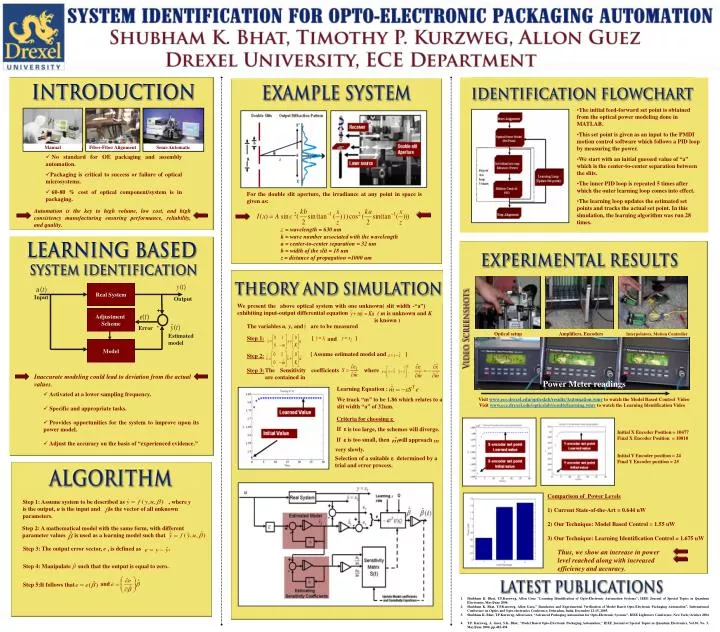
1. Real System Input Output + Adjustment Scheme - Error Estimated model Model Step 1: Assume system to be described as , where y is the output, u is the input and is the vector of all unknown parameters. Step 2: A mathematical model with the same form, with different parameter values is used as a learning model such that Step 3: The output error vector, e , is defined as . Step 4: Manipulate such that the output is equal to zero. = wavelength = 630 nm k = wave number associated with the wavelength a = center-to-center separation = 32 um b = width of the slit = 18 um z = distance of propagation =1000 um and Step5: Itfollows that Identification Flowchart Example System • The initial feed-forward set point is obtained from the optical power modeling done in MATLAB. • This set point is given as an input to the PMDI motion control software which follows a PID loop by measuring the power. • We start with an initial guessed value of “a” which is the center-to-center separation between the slits. • The inner PID loop is repeated 5 times after which the outer learning loop comes into effect. • The learning loop updates the estimated set points and tracks the actual set point. In this simulation, the learning algorithm was run 28 times. Manual Fiber-Fiber Alignment Semi-Automatic • No standard for OE packaging and assembly automation. • Packaging is critical to success or failure of optical microsystems. • 60-80 % cost of optical component/system is in packaging. For the double slit aperture, the irradiance at any point in space is given as: Automation is the key to high volume, low cost, and high consistency manufacturing ensuring performance, reliability, and quality. Experimental Results Theory and Simulation We present the above optical system with one unknown( slit width -“a”) exhibiting input-output differential equation ( m is unknown and K is known ) The variables u, y, and are to be measured Optical setup Amplifiers, Encoders Interpolators, Motion Controller { } Step 1: and { Assume estimated model and } Step 2: The Sensitivity coefficients are contained in where Step 3: Inaccurate modeling could lead to deviation from the actual values. Power Meter readings Learning Equation : • Activated at a lower sampling frequency. • Specific and appropriate tasks. • Provides opportunities for the system to improve upon its power model. • Adjust the accuracy on the basis of “experienced evidence.” Visit www.ece.drexel.edu/opticslab/results/Automation.wmv to watch the Model Based Control Video Visit www.ece.drexel.edu/opticslab/results/learning.wmv to watch the Learning Identification Video We track “m” to be 1.86 which relates to a slit width “a” of 32um. Criteria for choosing e If e is too large, the schemes will diverge. Initial X Encoder Position = 10477 Final X Encoder Position = 10810 Initial Y Encoder position = 24 Final Y Encoder position = 25 If e is too small, then will approach very slowly. Selection of a suitable e determined by a trial and error process. Algorithm • Comparison of Power Levels • Current State-of-the-Art = 0.644 uW • Our Technique: Model Based Control = 1.55 uW • Our Technique: Learning Identification Control = 1.675 uW Thus, we show an increase in power level reached along with increased efficiency and accuracy. • Shubham K. Bhat, T.P.Kurzweg, Allon Guez "Learning Identification of Opto-Electronic Automation Systems", IEEE Journal of Special Topics in Quantum Electronics, May/June 2006. • Shubham K. Bhat, T.P.Kurzweg, Allon Guez,” Simulation and Experimental Verification of Model Based Opto-Electronic Packaging Automation”, International Conference on Optics and Opto-electronics Conference, Dehradun, India, December 12-15, 2005. • Shubham K. Bhat, T.P.Kurzweg, Allon Guez, “Advanced Packaging Automation for Opto-Electronic Systems”, IEEE Lightwave Conference, New York, October 2004 . • T.P. Kurzweg, A. Guez, S.K. Bhat, "Model Based Opto-Electronic Packaging Automation," IEEE Journal of Special Topics in Quantum Electronics, Vol.10, No. 3, May/June 2004, pp.445-454.