Download
1 / 19
190 likes | 454 Views
Hash Tables. CSC220 Winter 2004-5. What is strength of b-tree? Can we make an array to be as fast search and insert as B-tree and LL?. Introduction of hash table. Data structure that offers very fast insertion and searching, almost O(1). Relatively easy to program as compared to trees.

E N D
Hash Tables CSC220 Winter 2004-5
What is strength of b-tree? • Can we make an array to be as fast search and insert as B-tree and LL?
Introduction of hash table • Data structure that offers very fast insertion and searching, almost O(1). • Relatively easy to program as compared to trees. • Based on arrays, hence difficult to expand. • No convenient way to visit the items in a hash table in any kind of order.
Hashing • A range of key values can be transformed into a range of array index values. • A simple array can be used where each record occupies one cell of the array and the index number of the cell is the key value for that record. • But keys may not be well arranged. • In such a situation hash tables can be used.
Converting Words to Numbers • Adding the digits :- Add the code numbers for each character. E.g. cats: c = 3, a = 1, t = 20, s = 19, gives 43. • What if, the Total range of word codes is from 1 to 260. • 50,000 words exist. • No enough index numbers. • Multiplying by powers :- Decompose a word into its letters. • Convert the letters to their numerical equivalents. • Multiply them by appropriate powers of 27 and add the results. • E.g. Leangsuksun = much larger than 260
Hash Function • Need to compress the huge range of numbers. • arrayIndex = hugenumber % smallRange; • This is a hash function. • It hashes a number in a large range into a number in a smaller range, corresponding to the index numbers in an array. • An array into which data is inserted using a hash function later is called a hash table.
Collisions • Two words can hash to the same array index, resulting in collision. • Open Addressing: Search the array in some systematic way for an empty cell and insert the new item there if collision occurs. • Separate chaining: Create an array of linked list of words, so that the item can be inserted into the linked list if collision occurs.
Open Addressing • Three methods to find next vacant cell: • Linear Probing :- Search sequentially for vacant cells, incrementing the index until an empty cell is found. • Clustering is a problem occurring in linear probing. • As the array gets full, clusters grow larger, resulting in very long probe lengths. • Array can be expanded if it becomes too full.
Quadratic Probing • load factor = nItems / arraySize; • If load factor isn’t high, clusters can form. • In quadratic probing more widely separated cells are probed. • The step is the square of the step number. • If index is x, the probe goes to x+1, x+4, x+9, x+16 and so on. • Eliminates primary clustering, but all the keys that hash to a particular cell follow the same sequence in trying to find a vacant cell (secondary clustering).
Double Hashing • Better solution. • Generate probe sequences that depend on the key instead of being the same for every key. • Hash the key a second time using a different hash function and use the result as the step size. • Step size remains constant throughout a probe, but its different for different keys. • Secondary hash function should not be the same as primary hash function. • It must never output a zero. • stepSize = constant – (key % constant); • Requires that size of hash table is a prime number.
Separate Chaining • No need to search for empty cells. • The load factor can be 1 or greater. • If there are more items on the lists access time is reduced. • Deletion poses no problems. • Table size is not a prime number. • Arrays (buckets) can be used at each location in a hash table instead of a linked list.
Hash Functions • A good hash function is simple and can be computed quickly. • Speed degrades if hash function is slow. • Purpose is to transform a range of key values into index values such that the key values are distributed randomly across all the indices of the hash table. • Keys may be completely random or not so random.
Random Keys • If the world were perfect, Evenly distributed NOT! • A perfect hash function maps every key into a different table location. • In most cases large number of keys are compressed into a smaller range of index numbers. • Distribution of key values in a particular database determines what the hash function needs to be. • For random keys: index = key % arraySize;
Non-random Keys • Consider a number of the form 033-400-03-94-05-0-535. • Every digit serves a purpose. The last 3 digits are redundant for error checking. • These digits shouldn’t be considered. • Every part of the remaining key should contribute to the data. • Use a prime number for the modulo base.
Folding • Break the key into groups of digits and add the groups. • The number of digits in a group should correspond to the size of the array.
Hashing Efficiency • Insertion and searching can approach O(1) time. • If collision occurs, access time depends on the resulting probe lengths. • Individual insert or search time is proportional to the length of the probe. This is in addition to a constant time for hash function. • Relationship between probe length (P) and load factor (L) for linear probing : P = (1+1 / (1 – L2)) / 2 for successful search and P = (1 + 1 / (1 – L))/ 2
Hashing Efficiency • Quadratic probing and Double Hashing share their performance equations. • For successful hashing : -log2(1 - loadFactor) / loadFactor • For an unsuccessful search :- 1 / (1 - loadFactor) • Searching for separate chaining :- 1 + loadFactor /2 • For unsuccessful search :- 1 + loadFactor • For insertion :- 1 +loadfactor ?2 for ordered lists and 1 for unordered lists.
Open Addressing vs. Separate Chaining • If open addressing is to be used, double hashing is preferred over quadratic probing. • If plenty of memory is available and the data won’t expand, then linear probing is simpler to implement. • If number of items to be inserted in hash table isn’t known, separate chaining is preferable to open addressing. • When in doubt use separate chaining
External Storage • Hash table can be stored in main memory. • If it is too large it can be stored externally on disk, with only part of it being read into main memory at a time. • In external hashing its important that the blocks do not become full. • Even with a good hash function, the block might become full. • This situation can be handled using variations of the collision-resolution schemes.