Download
1 / 29
290 likes | 423 Views
Angular regression. Louis-Paul Rivest S. Baillargeon, T. Duchesne, D . Fortin & A. Nicosia. Summary. 1- Animal movement in ecology 2- A general regression model for circular variable 3- Modeling the errors 4- Data analysis and simulation results.

E N D
Angular regression Louis-Paul Rivest S. Baillargeon, T. Duchesne, D. Fortin & A. Nicosia
Summary 1- Animal movement in ecology 2- A general regression model for circular variable 3- Modeling the errors 4- Data analysis and simulation results
Study the interaction between an animal and its environment using GIS data on land cover GPS data on animal motion Special software (ArGIS) is used to merge the data together Animal movement in ecology
Animal movement in ecology Target 1: meadow Dependent variable: yt motion angle at time t. Predicted value: (y| x1t , …) a compromise between several targets x1t Pt+1 Target 2: Canopy gap x2t yt Pt Pt-1 yt-1
Ecologists are uneasy about combining targets’ directions. McClintock et al. (Ecological Monograph 2012) define a compromise z,tbetween the angles t-1 and z,t as Animal movement Not right for a non integer z They are not fully satisfied with their definition. They add a word of caution: without providing details.
A general circular regression model Let (x1, z1),..., (xp, zp) be explanatory variables measured on each unit where x is an angle and z is a positive linear variable. The mean direction of y given (x1, z1),..., (xp, zp), (y|x, z), is the direction of
Motivating example: latent classes Mixture model: Each target is associated to a state. Given state j the conditional model for yiis xjiplus some errors The unconditional mean direction of yiis (y|x,z) with z=1 and jρj pj. ρj =E{cos(ε j )} is the mean resultant length of the deviations εj in state j
A general circular regression model Standardization: 1 = z1 =1. Examples (z=1): Mean direction model x1=0, and x2=/2 Rotation model x1=w, and x2=w+/2
A general circular regression model Examples (z=1): Decentred predictor (Rivest, 1997) x1=w, and x2=w+/2, x3=0, and x3=/2
A general circular regression model Presnell & all (1998) model: z1 = z2 =0, z3 = z4 =w, x1=0, x2=/2, x3=0, x4=/2, Jammalamadaka& Sen Gupta (2001) models. The Moebius model of Downs & Mardia (2002) does not belong!
Models for the errors We use the von Mises density for both specifications: with population MRL . This is a modified Bessel function
Modeling the errors von Mises variable Option 1 (homogeneity model): The density of does not depend on neither x nor z. It is von Mises with concentration parameter .
Modeling the errors von Mises variable Option 2 (Consensus, Presnell et al, 1998): The concentration parameter of is ℓ, where ℓ is the length of It is large when all the angles xj point in the same direction.
Modeling the errors The consensus model uses the parameters to model the mean direction and the concentration of the dependent angle y. Wouldn’t it be better to use two independent sets of parameters, one for the direction and one for the error concentration, (Fisher, 1992 mixed models)?
Models for the errors For the consensus model, the density of y given (x,z) is This is the conditional distribution for a multivariate von Mises model (Mardia, 1975). This density belongs to the exponential family and parameter estimation should be easy.
Parameter estimation Strategy: Maximize the von Mises Likelihood (use several starting values for the homogeneous errors) Use the inverse of the Fisher information matrix to approximate the sampling distributions of the estimates (model based) Calculate robust sandwich variance covariance matrices for the parameter estimates (valid even if the model assumptions are violated) Alternative estimation strategies: use the projected normal (Presnell & al., 1998) or the wrapped Cauchy as an error density.
Parameter estimation Score functions [i= (y|xi, zi)]: 1-Homegenous errors 2-Consensur errors (j=j, ℓi =ℓi)
Parameter estimation Data: (yi , xi , zi ), i=1,...,n Maximizing the von Mises likelihood with homogeneous errors leads to a max-cosine estimation criterion for the parameters {j}: Numerical problems may occur. Example: data simulated from the homogeneous error model: n=50, p=2, 2 =0.5 x1 =0, x2 U(-,), =0.4
Parameter estimation Properties: The max-cosine estimator for is consistent under the two error specifications, homogeneous and consensus; When the errors are homogeneous, the consensus MLE might not be consistent. A lack of robustness to the specifications of the errors’ distribution is the price to pay for the numerical stability of the likelihood.
Parameter estimation Properties: Bias: In a one parameter model with homogenoeus errors, the consensus MLE underestimates 2 (by up to 20%) MLE: The algorithm that maximizes the homogeneous likelihood must use several starting values (more that 1000!)
A time series model The conditional mean direction of yt is a compromise between yt-1 and x0 : Under consensus errors with von Mises distributions (Mardia et al, 2007) Stationary distribution unknown for homogeneous errors.
A time series model This is a “Biased Correlated Random Walk” in Ecology: yt= direction of animal movement at time t x0=x0t= direction of a target to which an animal might be attracted (“Directional Bias”) The estimation of 2 relies on the methods presented earlier.
Example 1: Periwinkle data y = direction of displacement x = distance traveled Presnell et al. (1998): projected normal errors Presnell et al fit Consensus fit Homogeneous fit: Numerical problems
yi = track orientation for pixel i x1i= track orientation for pixel i-1 x2i= angle for next meadow z2i= log(distance to next meadow) x3i= angle for next canopy gap z3i= log(distance to next canopy gap) Example 2: Dancose (2011) digitized bison track data K=218 trails for 5600 pixels Model considered
Model Bison track data: homegenous model estim. s.e.(R) s.e.(FI) beta2 1.06 0.10 0.05 S beta3 0.07 0.03 0.03 S beta4 -0.16 0.018 0.009 S beta5 -0.002 0.006 0.006 NS The tracks are “biased” towards target meadows (TM) and canopy gaps. When approaching a meadow, the bisons zoom in. The weight of the TM angle is 1-0.16 log(D)/1.06D-0.15.
Model Bison track data: consensus model estim Homo estimConsen se(FI) beta2 1.06 1.24 0.05 beta3 0.07 0.07 0.03 beta4 -0.16 -0.19 0.009 beta5 -0.002 -0.003 0.006 The two sets of estimates are similar and lead to the same conclusion.
Discussion • Multivariate angular regression applies beyond animal movement: • Meteo: ensemble prediction of wind direction • Experimental psychology: real and perceived orientation of features • Geophysics: direction of earthquake ground movement and direction of steepest descent • Thank you!
References • Dancose, K., D. Fortin, and X. L. Guo. 2011. Mechanisms of functional connectivity: the case of free-ranging bison in a forest landscape. Ecological Applications 21:1871-1885. • Downs, T. D. and Mardia, K. V. (2002) Circular regression. Biometrika,89,683-697 • Fisher, N.I., Lee A.J. (1992). Regression models for angular responses. Biometrics, 48, 665-677 • Fortin & al (2005) Wolves influence elk movements: behavior shapes a trophic cascade in Yellowstone National Park, Ecology, 86(5), 2005, pp. 1320–1330 • Jammalamadaka, S. R. and SenGupta, A. (2001) Topics in Circular Statistics. World Scientific: Singapour • Mardia, K.V. and Jupp, P.E. (1999) Directional Statistics,JohnWiley, New York • Presnell, B., Morrison, S.P., and Littell, R.C. (1998). Projected multivariate linear models for directional data. JASA. 93(443): 1068-1077 • Rivest, L.-P. (1997). A decentred predictor for circular-circular regression. Biometrika, 84, 717-726.