Download
1 / 36

E N D
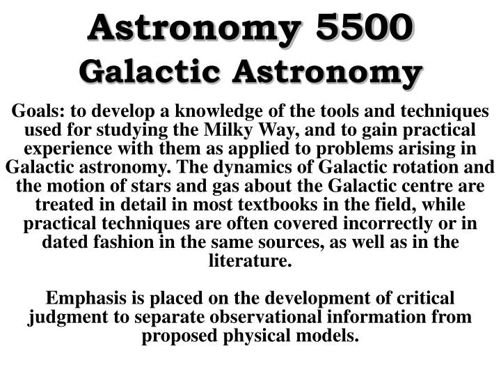
Astronomy 5500Galactic Astronomy Goals: to develop a knowledge of the tools and techniques used for studying the Milky Way, and to gain practical experience with them as applied to problems arising in Galactic astronomy. The dynamics of Galactic rotation and the motion of stars and gas about the Galactic centre are treated in detail in most textbooks in the field, while practical techniques are often covered incorrectly or in dated fashion in the same sources, as well as in the literature. Emphasis is placed on the development of critical judgment to separate observational information from proposed physical models.
1. Historical Landmarks The proper study of the Milky Way Galaxy probably begins in 1610, when Galileo first discovered that the Milky Way consists of “innumerable” faint stars. In 1718 Halley discovered the proper motions of Arcturus, Sirius, and Aldebaran, and by 1760 Mayer had published proper motions for some 80 stars based upon comparisons of their recorded positions. His results established that the Sun and stars are not at rest relative to one another in the Galaxy. The obvious problem with trying to map our Galaxy from within is that the Sun is but one of many billions of stars that populate it, and our vantage point in the disk 8-9 kpc from the Galactic centre makes it difficult to detect objects in regions obscured by interstellar dust. But attempts have been made frequently.
In 1785 William Herschel derived the first schematic picture of the Galaxy from optical “star gauging” in 700 separate regions of the sky. He did it by making star counts to the visual limit of his 20 foot (72-inch diameter) telescope. He assumed that r ~ N1/3 (i.e. N ~ r3), and obtained relative thicknesses for the Galactic disk in the various directions sampled. No absolute dimensions were established. By 1817 Hershel had adopted a new picture of the Galaxy as a flattened disk of nearly infinite extension (similar to the modern picture).
In 1837 Argelander, of the Bonn Observatory and orginator of the BD catalogue, was able to derive an apex for the solar motion from studying stellar proper motions. His result is very similar to that recognized today. Also in 1837, Frederick Struve found evidence for interstellar extinction in star count data, which was considered necessary at that time to resolve Herschel’s “infinite universe” with Olber’s paradox (which had been published in 1823). By the turn of the century many astronomers felt that a concerted, detailed effort should be made to establish reliable dimensions for the Milky Way. The task was initiated by Kapteyn in 1905 with his plan to study in a systematic fashion 206 special areas, each 1° square, covering most of the sky — the well known “Selected Areas” for Galactic research. By then, separately-pursued research programs into the nature of the Milky Way system often produced distinctly different results.
In 1918, for example, Shapley noted the asymmetric location of the centre of the globular cluster system with respect to the Sun, and suggested that it coincided with the centre of the Galaxy. But the distance to the Galactic centre found in such fashion was initially overly large because of distance scale problems. Longitude distribution of globular clusters.
Kapteyn and van Rhijn published initial results from star counts in 1920, namely a Galaxy model with a radius of ~4.5 kpc along its major plane and a radius of ~0.8 kpc at the poles. Kapteyn published an alternate model in 1922 in with the Sun displaced from the centre, yet by less than the distance of ~15 kpc to the centre of the globular cluster system established by Shapley.
The issue reached a turning point in 1920 with the well known Shapley-Curtis debate on the extent of the Galactic system. The merits of the arguments presented on both sides of this debate have been the subject of considerable study over the years, but it was years later before the true extragalactic nature of the spiral nebulae was recognized. Although Shapley was considered the “winner” of the debate, it was Curtis who argued the correct points. A big step was Hubble’s 1924 derivation of the distance to the Andromeda Nebula using Cepheid variables. Somewhat less well-known is Lindblad’s 1926 development of a mathematical model for Galactic rotation. Lindblad’s model was developed further in 1927-28 by Oort, who demonstrated its applicability to the radial velocity data for stars. Finally, in 1930 Trumpler provided solid evidence for the existence of interstellar extinction from an extremely detailed study of the distances and diameters of open star clusters.
The modern era orginated in 1944 when Baade published his ideas on different stellar populations. In 1940 during World War II, Grote Reber had discovered the radio radiation from the Galactic centre, but it was not until after the end of the war that the discovery was pursued by research groups in The Netherlands (Müller and Oort), the U.S. (Ewen and Purcell), and Australia (Christiansen), often making use of radio dishes left behind by German occupation forces. The prediction and confirmation of the 21-cm transition of neutral hydrogen in the Galactic disk initiated the new specialty of radio astronomy, and led to a boom era in the study of our Galaxy. Although less popular now than it was 30 years ago, Galactic astronomy is still an important area of study.
Perhaps the best “picture” of the Galaxy is that sketched by Sergei Gaposhkin from Australia, as published in Vistas in Astronomy, 3, 289, 1957. The lower view is Sergei’s attempt to step outwards by 1 kpc from the Sun.
Sergei Gaposhkin’s drawing is crucial for the insights it provides into the size and nature of the Galactic bulge, that spheroidal (or bar-shaped?) distribution of stars surrounding the Galactic centre. Keep in mind that all such attempts rely heavily upon the ability of the human eye (and brain) to distinguish a “grand design” from the confusing picture posed by the interaction of dark dust clouds, bright gaseous nebulae, and rich star fields along the length of the Milky Way (see below).
2. Current Model of the Galaxy The present picture of the Galaxy has the Sun lying ~20 pc above the centreline of a flattened disk, ~8±0.5 kpc from the Galactic centre. The spheroidal halo is well established, but the existence of a sizable central bar and the nature of the spiral arms are more controversial.
Another schematic representing the present view of the Galaxy.
An alternate picture of the Galaxy from the instructor in recent years has the Sun lying ~20 pc above the centreline of a flattened disk, ~8±1 kpc from the Galactic centre. The spheroidal halo is well established, and there is an obvious warping of the Galactic disk in the direction of the Magellanic Clouds that is best seen in the fourth Galactic quadrant.
Best current estimates for the distance of the Sun from the Galactic centre tend to cluster around ~8 ±1 kpc = R0, although that is not well-established. Estimates as low as ~6.5 kpc and as high as ~10.5 kpc have been published. The main components of the Galaxy are the bulge, the disk (which contains the spiral arms), and the halo, with some debate about the exact number of subgroups of them. The existence of a bar at the Galactic nucleus is accepted from indirect evidence only. There is considerable evidence for a metallicity gradient in the disk with stars of higher metallicity lying towards the Galactic centre. The metal enrichment of the disk is attributed to evolutionary processes in stars, which end their lives by adding a rich supply of heavy elements to the interstellar medium.
When the mean metallicity of disk stars is studied as a function of the age of the stars, there appears to be a net metallicity growth with age amounting to: Δ<[Fe/H]> ≈ 0.5–0.7/1010 years, i.e. an increase of Fe/H by 4 ±1 every 1010 years. The relationship is not zeroed to the Sun, since solar metallicity is calculated to have been reached at an age of ~2.5 109 years. [Fe/H] = log[(Fe/H)/(F/H)], i.e. 2 the solar metallicity is equivalent to [Fe/H] = +0.30. Of the main components of the Galaxy, there are at least two components of the halo currently recognized, as well as some argument about the number of disk components that can be identified (thin disk, thick disk, etc.). The components of spiral arms appear to differ only slightly in age, and many astronomers would identify them as a single young Population I component.
Table 24.1 from Carroll and Ostlie. Approximate Values for Parameters Associated with Components of the Milky Way.
Well-recognized characteristics of the Galaxy: 1. Gould’s Belt, consisting of nearby young stars (spectral types O and B) defining a plane that is inclined to the Galactic plane by 15 to 20. Its origin is uncertain. The implication is that the local disk is bent or warped relative to the overall plane of the Galaxy. This is not to be confused with the warping of the outer edges of the Galaxy.
2. An abundance gradient exists in the Galactic disk and halo, consistent with the most active pollution by heavy elements occurring in the densest regions of these parts of the Galaxy. See results below from Andrievsky et al. A&A, 413, 159, 2004 obtained from stellar atmosphere analyses of Cepheid variables.
The abundance gradient is also seen in the halo according to the distribution of globular clusters of different metallicity relative to the Galactic centre (below).
3. The orbital speed of the Sun about the Galactic centre is about 250 km s–1, as determined from the measured velocities of local group galaxies, as well as from a gap in the local velocity distribution of stars corresponding to “plunging disk” stars. This fact is actually NOT “well recognized” by most astronomers.
4. The Galactic bulge is spheroidal, although some researchers believe it displays a boxy structure at infrared wavelengths suggestive of a central bar viewed nearly edge on. A mapping (right) of Milky Way planetary nebulae in Galactic co-ordinates (Majaess et al. MNRAS, 398, 263, 2009) suggests a more spheroidal structure typical of galaxies like NGC 4565 (top). The nature of the Galactic bulge is still unclear. The surface brightness follows a de Vaucouleurs law.
5. The Galaxy is a spiral galaxy. But does it have 2 arms or 4, and can it be matched by a logarithmic spiral? A “grand design” spiral pattern is not obvious in the plot of the projected distribution of Cepheids (points) and young open clusters (circled points) below (Majaess et al. 2009).
A schematic representation of what are considered to be major spiral features. How would you connect the points? Most recent studies consider the Cygnus feature to be a spur or minor arm, and the Perseus feature is considered to be a major arm! There is an “Outer Perseus Arm” in many deep surveys. It lies >4 kpc from the Sun In the direction of the Galactic anticentre.
6. The Galactic disk is warped, presumably from a gravitational interaction with the Magellanic Clouds. The warp is evident in 21cm maps of neutral hydrogen restricted (by radial velocity) to lie at large distances from the Galactic centre (below).
7. The Galaxy has a magnetic field that appears to be coincident with its spiral arms (or features), with the likely geometry of the magnetic field lines running along the arms. Weak fields of ~tens of mGauss are typically measured. The evidence for the presence of a magnetic field comes from the detection of interstellar polarization in the direction of distant stars (see below).
8. Note features in Carroll and Ostlie that are NOT included in the list: spiral structure the Milky Way’s central bar 3-kpc expanding arm dark matter halo evidence of dark matter Can you understand why?
3. Stellar Reference Frames and Proper Motions If we define the equatorial coordinates of a star to be α1 and δ1 at epoch T1, and α2 and δ2 at epoch T2, then: α2 – α1 = (m + n sin α tan δ + μα)(T2 – T1) and δ2 – δ1 = (n cos α + μδ)(T2 – T1), where m and n are the terms for general precession. As determined by Newcomb with respect to observations of planets and asteroids, with known (or estimated) masses of solar system objects used to establish a dynamical rest frame, the “constant” of luni-solar precession is given by: p = 50".2910 + 0".0222 T per year, where T is the number of elapsed centuries since J2000.0, i.e. p = 50".2688 per year for the year J1900.0. Thus, for example: p(1985.0) = 50".2910 – 0".0222 (85.0/100) per year = 50".27213 per year.
General precession consists of two terms: p1 = luni-solar precession, and λ = planetary precession (a function of α only). Thus, m = p1 cos ε– λ = 3s.07496 + 0s.00186T /year, and n = p1 sin ε = 1s.33621 – 0s.00057T /year = 20".0431 – 0".0085T /year, where ε is the obliquity of the ecliptic. The parameters μα and μδ are the proper motions in right ascension and declination, respectively. In other words: and the net proper motion of an object is given by μ = [(μα cos δ)2 + μδ2]½. Accurate proper motions for stars therefore require small internal errors of observation as well as a detailed knowledge of the inertial reference frame and the resulting precession constants (which are not well determined).
The steps usually taken to determine reliable proper motions for stars are: (i) Meridian telescopes and accurate clocks are used to establish reliable position measurements for bright stars, with stellar observations also being used (if possible) to establish the location of the celestial pole for the epoch of the observations. (ii) The current right ascensions and declinations for all program stars are obtained from repeated measurements of each star’s meridian crossing times as well as its culmination points measured on the telescope’s large altitude circle. (iii) Published precession and nutation constants are used to reduce the observations to a common nearby epoch in time, and the results are published as a Catalogue of Stellar Positions.
(iv) Several such catalogues are reduced to a common epoch to establish the proper motions, systematic observatory errors, systematic precession constant errors, etc. for a common set of stars. The resulting collection of positions and proper motions is a Compilation Catalogue. (v) When several such catalogues are combined with a new set of planetary observations used to redefine the inertial reference frame for the precessional corrections, the resulting compilation of positions and motions tied to the inertial reference frame is known as a Fundamental Catalogue, e.g. the FK4 and FK5. (vi) Proper motion data for stars in Position Catalogues but not in a Fundamental Catalogue are obtained by establishing Catalogue corrections tied to the Fundamental Catalogue reference frame. Several such “non-fundamental” catalogues exist, of which the SAO Catalogue and AGK3 are two examples.
A simple way of assessing the problem of deriving reliable proper motions for stars is to consider the various sources of error involved: The proper motion of a star in a fundamental catalogue, μF, is given by: μF = P + S + G + (μ + σF + εF) , where: P = the effect arising from an error in precession, S = the effect caused by the solar motion, G = the effect resulting from galactic rotation, μ = the residual motion of the star after removal of P, S and G (i.e. the star’s space motion), σF = the systematic error in the fundamental system (always a possibility!), and εF= the accidental error for a particular star.
Usually, catalogued μF values are used for as many stars as possible, distributed at random in position and magnitude, to remove μ, σF, and εF from discussion. Any subsequent analyses of μF values to derive S and G may therefore contain an error caused by P. In fact, evidence for a residual error in precession for the FK4 system (i.e. P > 0) was the primary motivation behind the studies leading to the production of the FK5 Catalogue. A possible alternate route is to use galaxies as reference objects for the positions of stars, which is possible for astronomical imaging. In that case the proper motion of a star, μG, measured in such fashion relative to galaxies, is given by: μG = S + G + (μ + σG + εG) , with the symbols as given previously. Proper motions obtained in such fashion do not involve uncertainties in the precession corrections.
The resulting differences in proper motion are: μF–μG = P + (σF – σG + εF– εG). Thus, analyses of large numbers of stars measured by both techniques can be used to establish P, provided that the terms in brackets are completely randomized. The potential advantages of measuring stars relative to galaxies was realized in the ‘50s and ‘60s, and led to the development of two observatory programs to test the concept. A Lick Observatory program (Vasilevskis) used the 0.5-m astrograph with 6° 6° photographic plates, and typically ~60 galaxies per field (to ~19th magnitude). The galaxies (faint and fuzzy) were used to establish plate constants, the correct orientations, etc., with limited success. A Pulkovo Observatory program (Fatchikin) used the normal astrograph with 2° 2° plates, and typically only 1 or 2 bright galaxies (to ~9th magnitude) per field. The galaxies were used to standardize the plates, with stars on the plates used to establish the reference system, plate constants, etc.
The Pulkovo program results were clearly based on a different standardization from that used in the Lick program. A Yale-Columbia program was a southern replication of the Lick program using an 0.5-m astrograph with 6° 6° plates, but also with superior optics to the Lick and Carnegie astrographs. Hanson (AJ, 80, 379, 1975; IAU Symp., 85, 71, 1980) used some of the Lick program plates for the central (and later outer) regions of the Hyades cluster field for his Ph.D. thesis study of the Hyades cluster distance based upon proper motions. The study was heavily criticized by Luyten (Publ.Univ.Minnesota, XLI, 1975), who argued that the technique suffers from the non-stellar nature of the galaxy images, which assures that stars and galaxies in the fields are measured in completely different ways. He suggested an alternative method of tying the measurements to quasar images, although that may not be practical for fields like the Hyades.
Uncertainties in proper motion measurements are typically of order ±0".005 /year to ±0".010 /year, although the results of the Hipparcos mission have generated stated precisions closer to ±0".001 /year . Proper motion studies are also made for open and globular clusters, where they are used to study membership probabilities for cluster stars or space motions of the clusters. In the case of membership testing, membership discrimination is based upon the analysis of proper motions relative to some inferred field star distribution. Recent variants use each star’s position in the cluster, in addition to proper motion, to specify membership.
An example of proper motions used to establish membership probabilities for stars in the open cluster M11 (McNamara et al. A&AS, 27, 117, 1977).