Download
1 / 8
80 likes | 87 Views
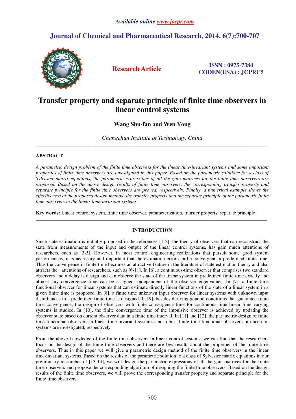
A parametric design problem of the finite time observers for the linear time-invariant systems and some important<br>properties of finite time observers are investigated in this paper. Based on the parametric solutions for a class of<br>Sylvester matrix equations, the parametric expressions of all the gain matrices for the finite time observers are<br>proposed. Based on the above design results of finite time observers, the corresponding transfer property and<br>separate principle for the finite time observers are proved, respectively. Finally, a numerical example shows the<br>effectiveness of the proposed design method, the transfer property and the separate principle of the parametric finite<br>time observers in the linear time-invariant systems.

E N D
Available online www.jocpr.com Journal of Chemical and Pharmaceutical Research, 2014, 6(7):700-707 ISSN : 0975-7384 CODEN(USA) : JCPRC5 Research Article Transfer property and separate principle of finite time observers in linear control systems Wang Shu-fan and Wen Yong Changchun Institute of Technology, China _____________________________________________________________________________________________ ABSTRACT A parametric design problem of the finite time observers for the linear time-invariant systems and some important properties of finite time observers are investigated in this paper. Based on the parametric solutions for a class of Sylvester matrix equations, the parametric expressions of all the gain matrices for the finite time observers are proposed. Based on the above design results of finite time observers, the corresponding transfer property and separate principle for the finite time observers are proved, respectively. Finally, a numerical example shows the effectiveness of the proposed design method, the transfer property and the separate principle of the parametric finite time observers in the linear time-invariant systems. Key words: Linear control system, finite time observer, parameterization, transfer property, separate principle _____________________________________________________________________________________________ INTRODUCTION Since state estimation is initially proposed in the references [1-2], the theory of observers that can reconstruct the state from measurements of the input and output of the linear control systems, has gain much attentions of researchers, such as [3-5]. However, in most control engineering realizations that pursuit some good system performances, it is necessary and important that the estimation error can be convergent in predefined finite time. Thus the convergence in finite time becomes an attractive feature in the literature of state estimation theory and also attracts the attentions of researchers, such as [6-11]. In [6], a continuous-time observer that comprises two standard observers and a delay is design and can observe the state of the linear system in predefined finite time exactly and almost any convergence time can be assigned, independent of the observer eigenvalues. In [7], a finite time functional observer for linear systems that can estimate directly linear functions of the state of a linear system in a given finite time is proposed. In [8], a finite time unknown input observer for linear systems with unknown input disturbances in a predefined finite time is designed. In [9], besides deriving general conditions that guarantee finite time convergence, the design of observers with finite convergence time for continuous time linear time varying systems is studied. In [10], the finite convergence time of the impulsive observer is achieved by updating the observer state based on current observer data in a finite time interval. In [11] and [12], the parametric design of finite time functional observers in linear time-invariant systems and robust finite time functional observers in uncertain systems are investigated, respectively. From the above knowledge of the finite time observers in linear control systems, we can find that the researchers focus on the design of the finite time observers and there are few results about the properties of the finite time observers. Thus in this paper we will give a parametric design method of the finite time observers in the linear time-invariant systems. Based on the results of the parametric solution to a class of Sylvester matrix equations in our preliminary researches of [13-14], we will design the parametric expressions of all the gain matrices for the finite time observers and propose the corresponding algorithm of designing the finite time observers. Based on the design results of the finite time observers, we will prove the corresponding transfer property and separate principle for the finite time observers. 700
Wang Shu-fan and Wen Yong J. Chem. Pharm. Res., 2014, 6(7):700-707 ______________________________________________________________________________ PROBLEM FORMULATION Consider the linear time-invariant system in the following form ( ) ( ) ( ), ( ) ( ) ( ) y t Cx t = x∈ℜ , and respectively; A , B Assumption A1: rank( ) Assumption A2: The matrix pair ( , rank sI A C n − = , s Consider a pair of observers of system (1) ( ) ( ) ( ) ( ) i i i i z t A LC z t L y t Bu t = − + + & n q iL ∈ℜ are the gain matrices and ( ) ( ) ( ) z t The pair of observers (2) can be written in the following compact form ( ) ( ) ( ) ( ) z t Nz t Ly t Hu t = + + & (3) 0 0 N , Assume that the state estimation of system (1) via observer (3) is designed as follows ˆ( ) [ ( ) ( )] x t M z t e z t D = − − (5) where 0 is a suitable chosen finite time. Definition 1. Given the linear time-invariant system (1) satisfying Assumptions A1 and A2. If there exist constant n q iL ∈ℜ ( ) in (2) or L in (3) and ˆ ( ) ( ) ( ) e t x t x t = − (6) can be convergent to zero in a finite time D and stays bounded during the convergence interval observer system (2) with (5), or the observer system (3) with (5) is called as a finite time observer of the linear time-invariant system (1). Theorem 1[6]. Given the linear time-invariant system (1) satisfying Assumptions A1 and A2. Problem DPFO has a = + x t & Ax t Bu t = ≥ , x t x t t 0 0 0 (1) y∈ℜ q u∈ℜ n p where are the state vector, the input vector and the output vector, q n × ∈ℜ are known matrices satisfying two assumptions as n n × n p × ∈ℜ ∈ℜ C and = = and rank( ) B p C q ; ) A C is observable, that is T T ∀ ∈ = ≥ ( ), 1,2, i t t (2) 0 × iz ∈ℜ, n i = 1,2 where are the state of the observers. Set z t 1 = z t 2 , , N L L B B 1 1 = = = N L H = − N A LC Where (4) 2 2 i i ND D > × i = 2n q × × 1,2 ∈ℜ ∈ℜ 2 n n M gain matrices in (5) such that the estimation error + [ ] t t D , the 0 0 exists. In addition, I I n = T − 1 ND T e T N( i = 1,2 solution, if and only if the matrices there holds [ 0 n n M I T = ) are Hurwitz and with n i − ] 1 ND e T (7) 701
Wang Shu-fan and Wen Yong J. Chem. Pharm. Res., 2014, 6(7):700-707 ______________________________________________________________________________ Based on the existing condition of finite time observers for linear systems in Theorem 1, the design problem of parametric design, transfer property and separate principle problem for the finite time observers in linear time-invariant systems can be described as follows, which can be denoted by Problem DPFO. Problem DPFO (Design of Parametric Finite-time Observers). Given the linear time-invariant system (1) satisfying Assumption A1 and Assumption A2. If the finite time observers (2) with (5) or (3) with (5) exits, determine the n q iL ∈ℜ ( such that the estimation error (6) converges to zero in a finite time D and stays bounded during the convergence [ ] t t D + for a suitable chosen finite time delay D. And then based on the above design results of finite time observers, prove the transfer property and separate principle for the finite time observers in linear time- invariant systems. SOLUTION TO PROBLEM DPFO iL, AND M × i = 2n q × × 1,2 ∈ℜ ∈ℜ 2 n n L M parametric expressions of the gain matrices ) in (2) or in (3), and in (5) interval 0 0 i = 1,2 1) SOLUTIONS TO MATRICES N, i = 1,2 Without loss of generality, we assume that the Hurwitz matrices have distinct and self-conjugate T i N by i kis ∈, and eigenvalues. We denote the eigenvalues and their corresponding eigenvectors of matrices n ki v ∈ ( L , ), respectively. Then there exist ( ) i ki i ki ki ki N v A LC v s v = − = , ( L Denote ( 1 2 diag , , , i i i ni s s s Λ = L , and [ ] i i i ni V v v v = L , By writing (8) into a compact form, we can obtain T T i i i i A V C W V − = Λ, (9) T i i i W L V = , (10) Further, equation (9) can be written into the following matrix form v s I A C w , L Based on the dual theory, the matrix pair ( , ) i = = 1,2 1,2, , k n T T i = = 1,2 1,2, , k n , )(8) ) i = 1,2 i = 1,2 1 2 i = 1,2 i = 1,2 where − = ki T T 0 n n × ki i = = 1,2 1,2, , k n ki , (11) T T A Cis observable is equivalent with that the matrix pair ( ( ) [ ] N s s ∈ℜ , ) A C is n q × q q × ∈ℜ ( ) [ ] s D s controllable. Therefore, there exist two polynomial matrices ( ) 0 ( ) D s , and such that N s − = T T sI A C ∀ ∈(12) s g ∈ q = 1,2, , k n L Comparing (11) with (12), we know that there must exist a group of parametric vectors 1,2 i = ) such that[13-14] ( ) ( ) ki ki w D s , L , ( , ki v N s ki ki = g ki i = = 1,2 1,2, , k n (13) 702
Wang Shu-fan and Wen Yong J. Chem. Pharm. Res., 2014, 6(7):700-707 ______________________________________________________________________________ iV and W, ( i = 1,2 Based on equations (10) and (13), we can give the parametric expressions of ( ) ( ) i i i i i V N s g N s g = L and ( ) ( ) i i i i i W D s g D s g = L Based on (10), (14) and (15), we can obtain 1 ( )T i i i L WV− = , (16) ) in (9) as i ( ) N s g i = 1,2 1 1 2 2 ni ni , (14) ( ) D s g i = 1,2 1 1 2 2 ni ni , (15) i = 1,2 g ∈ q iL ( i = = 1,2 1,2, , k n L In order to guarantee that the gain matrices 1,2 i = ) must satisfy the following constraint: s s = ND T e T [ 0 n n n n M I T × × = where the matrix e can be parameterized by diag( , ) diag e V V = ) are real, the free parameter vector ( , ki ⇔ = = = , , 1,2, , , n i 1,2 g g l k L Constraint C1. ki li ki li is inverted, from (7) and (14) we can obtain the parametric expression of × ∈ℜ 2 n n M If the matrix as − ] 1 ND e T (17) ND ( ) Λ Λ − D D 1 ND T T T T , diag( , ) e e V V 1 2 1 2 1 2 (18) iV, i = 1,2 and 2) TRANSFER PROPERTY OF THE FINITE TIME OBSERVERS Theorem 2. Given the linear time-invariant system (1) satisfying Assumption A1 and Assumption A2. Then there holds that the closed-loop transfer function of system (1) under state feedback observer (2) with (5) or (3) with (5) is equal to that of system (1) under state feedback u Proof. The closed-loop system of system (1) under state feedback u ( ) ( ) ( ) ( ) ( ) ( ) y t Cx t = (19) It is easy to obtain its closed-loop transfer function as follows 1 ( ) [ ( )] W s C sI A BK B = − + (20) The closed-loop system of system (1) under state feedback with (5) can be given by ( ) ( ) ( ) ( ) ( ) ( ) ( ) ( ) ( ) ( ) ( ) z t N HKM z t LCx t HKMe z t D Hv t = + + − − + & We can rewrite (21) into a matrix form as follows are determined by (14). = + ˆ u Kx Kx = v of the finite time v . + = + Kx v can be given by = + + x t & A BK x t Bv t − = + ˆ u Kx v of the finite time observer (2) with (5) or (3) = + − − + ND x t & Ax t BKMz t BKMe z t D Bv t ND (21) 703
Wang Shu-fan and Wen Yong J. Chem. Pharm. Res., 2014, 6(7):700-707 ______________________________________________________________________________ ( ) ( ) z t & ( ) ( ) z t x t & A BKM HKM + x t = LC N B H ND BKMe HKMe − − + ( ) ( ) v t z t D ND (22) By using the Laplace transform to (22), we can obtain ( ) ( ) Z s LC N HKM + + Then system (23) can be written in a simple form as A BKM BKMe LC N HKM HKMe + − Denote 0 I P T I , Based on (7), we can obtain A BKM BKMe Q LC N HKM HKMe + − = − + = − − + − = − A BKMT BKMe LC TA NT − + + − = and B B Q H , Under the transformation the closed-loop system (21) or (24) is equivalent with the following system B A BK BKM BKMe e C N − − ( ) ( ) ND Ds X s X s Z s A BKM BKMe HKMe − e = s − ND Ds e B H ( ) V s (23) (24) − − ND Ds B H e [ ] , , 0 C − ND Ds e 0 I I T = = Q − − − ND Ds e P − ND Ds e − − ND Ds 0 I 0 I I T I A BKM HKM BKMe HKMe − e − ND Ds T LC N e − − 0 I ND Ds I T A BKM BKMe N + e − − + − ND Ds ND Ds LC TA TBKM TBKMe e HKM HKMe e − ND Ds 0 I I A BKM BKMe N e T LC TA − − + − − ND Ds ND Ds e T BKM BKMe N e = − ND Ds A BK BKM BKMe N e 0 , = [ ] 0 = C P C 0 c (25) − + − ND Ds [ ] , , 0 0 0 704
Wang Shu-fan and Wen Yong J. Chem. Pharm. Res., 2014, 6(7):700-707 ______________________________________________________________________________ It is easy to find that the transfer function of the closed-loop system (21) or (24) is same with that of (25), and the transfer function of (25) is equal to (20), which is the transfer function of (19), because the following result holds: 1 0 0 0 N − + = − = − + 3) SEPARATE PRINCIPLE OF THE FINITE TIME OBSERVERS Theorem 3. The eigenvalues of the closed loop system for the linear time-invariant system (1) via the state feedback ˆ u Kx v = + of the finite time observer (2) with (5) or (3) with (5)) are equal to the sum of the eigenvalues ( ) A BK λ + of the closed loop system for the linear time-invariant system (1) via state feedback u ( ) N λ of the finite time observer. Proof. From the proof of Theorem 2, there holds ND Ds A BK BK A BKM BKMe e Q P N LC N HKM HKMe e + − , A BKM BKMe A LC N HKM HKMe + − there holds ( ) ( ) ( ) A BK N λ λ λ = + U . A NUMERICAL EXAMPLE Consider the linear system (1) with the following parameters as 2 1 1 0 1 1 0 0 3 − , It is easy to see that the matrix pair ( , ) − − + − ND Ds B A BK BKM BKMe e [ ] − C sI ][ ] − 1 ( ) * sI A BK B [ 0 C ( ) − 0 1 0 sI N [ ] − 1 ( ) C sI A BK B = + Kx v and the eigenvalues + − − = − 0 ND Ds is equivalent with the matrix A − − ND Ds e = c − ND Ds e + BK We can know that the matrix , thus cA − 0 1 1 = − = , A B 1 0 0 1 0 0 = C A C is observable. Thus we can utilize the proposed parametric design ( ) ( ) N sand D ssatisfying method of finite time observers in this example. We can calculate the polynomial matrices (24) as 3 1 ( ) 0 1 1 0 , + − s = − − − + 2 N s 5 6 2 s s s = ( ) D s + − − 3 2 s s s = −, = − + 2 1 8 N, s j i = 1,2 For simplicity, we select the eigenvalues of the Hurwitz matrices 1 8 s j = − − and , 2 1 , We can obtain by , i 11 21 s = − = − + = − − 10 3 3 3 3 s j s j , , respectively, and 31 12 22 32 − + − − + − − , , , , 2 3 1 6 + 2 3 1 6 − 3 1 2 6 5 + 1 2 6 5 − j j j j j j = = = = = = g g g g g g 11 21 31 12 22 32 − 2 j j 705
Wang Shu-fan and Wen Yong J. Chem. Pharm. Res., 2014, 6(7):700-707 ______________________________________________________________________________ − − 4.0074 26.4113 19.2167 0.8744 2.0074 3.3153 = L 1 and 8.7849 13.948 14.2695 0.208 1.2151 10.2057 − = L 2 By selecting D = 0.8 , we can obtain − − − − 0.1452 1.6752 1.5072 0 0 0 0.2855 0.0662 1.8578 0.1332 0.2285 0.1619 0 0 0 0.0089 0.0744 0.0189 0.0601 0.1548 0.314 0 0 0 0 0 0 0 0 0 0 0 0 = ND e − 0.1379 0.151 0.9897 − 0.7145 0.0662 1.8578 − 0.0759 0.0674 0.524 0.0089 1.0744 0.0189 − 0.0035 0.0407 0.0022 − 0.0495 0.1151 0.612 − − − − − 0.0495 0.1151 0.338 = − − M Substituting the above matrices into the finite time observer (2) with (5) or (4) with (5), we finish the design of the finite time observer. ( ) sin u t t = is the input signal of the system (1), [1 2 4 5 7 8]T z = is the initial state of the finite time observer. By using the function ODE45 in Matlab, we can give the simulation figure to compare the state of system (1) and the finite time observer with 0.8 D = in Fig. 1. From Fig. 1, we can find that the errors between the linear system and the designed finite time observer almost converges to zero in the finite time 0.8 x = − 1]T [1 2 Assume that is the initial state of the system (1) 0 and 0 D = . 1 observer system the first components 0.5 0 -0.5 0 1 2 3 4 5 6 t/sec D = 0.8 Figure 1. The first state components of the linear system and the finite time observer with In addition, we select the eigenvalues of the closed-loop system for system (1) under state feedback u 6 7i − + , 6 7i and 4 − . The corresponding gain matrix of state feedback is obtained as [ 130 56 66] K = − − By Theorem 2, the closed-loop transfer functions of both system (1) under state feedback time observer (2) with (5) or (3) with (5) and system (1) under state feedback u = Kx as − − = + ˆ u Kx v of the finite = + Kx v are 706
Wang Shu-fan and Wen Yong J. Chem. Pharm. Res., 2014, 6(7):700-707 ______________________________________________________________________________ + + + + 2 283 4 283 s + + 3 2 72 2 s s s s + + 3 2 72 2 s s s And by Theorem 3, the eigenvalues of the closed-loop system for the linear time-invariant system (1) via the state feedback ˆ u Kx v of the finite time observer (2) with (5) or (3) with (5)) are same with the sum of the ( ) A BK λ + of the closed loop system for the linear time-invariant system (1) via state feedback u Kx v = + and the eigenvalues of the finite time observer, which can be given by { 6 7 , 4, 1 8 , 10, 3 3 i j j − ± − − ± − − ± . CONCLUSION In this paper the design problem and its properties of a finite time observer for linear time-invariant systems is studied. The proposed finite time observer merges the advantages of the individual observers, such as finite time convergence. And the transfer property and separate principle for the finite time observers are still held for the finite time observers. Finally, the parametric design method of the finite time observer has been demonstrated on a numerical example and the simulation results show that this parametric design method, transfer property and separate principle for the finite time observers are effective. REFERENCES [1]R. E. Kalman, R.S. Bucy. ASME Journal of Basic Engineering, Vol. 83D, 95–108, 1961. [2]D. G. Luenberger. IEEE Transactions on Military Electronics, Vol. 8, 74–80, 1964. [3]S. Barnett. Introduction to mathematical control theory, Clarendon Press, Oxford, UK, 1975. [4]T. Kailath. Linear systems, Prentice-Hall Press, Upper Saddle River, NJ, 1985. [5]J. O’Reilly. Observers for linear systems, Academic Press, New York, US, 1983. [6]R. Engel, G. Kreisselmeier. IEEE Transactions on Automatic Control, Vol. 47, 202-1204, 2002. [7]T. Raff, P. Menold, C. Ebenbauer, F. Allg¨ower. A finite time functional observer for linear systems. Proceedings of the 44th IEEE Conference on Decision and Control, and the European Control Conference, 7198-7203, 2005. [8]T. Raff, F. Lachner, F. Allg¨ower. A finite time unknown input observer for linear systems. 14th Mediterranean Conference on Control and Automation, 1-5, 2006. [9]P. H. Menold, R. Findeisen, F. Allg¨ower. Finite time convergent observers for linear time varying systems. Proceedings of the 11th Mediterranean Conference on Control and Automation, 212-217, 2003. [10]T. Raff, F. Allg¨ower. An impulsive observer that estimate the exact state of a linear continuous-time system in predetermined finite time. Proceedings of the 11th Mediterranean Conference on Control and Automation, 1-3, 2007. [11]L. B. Zhao, G. S. Wang. Design of Finite Time Functional Observers in Linear Control Systems. 2012 Third International Conference on Intelligent Control and Information Processing, July 15-17, 2012 - Dalian, China, pp. 303-307 [12]G. S. Wang, W. L. Yang, Q. Lv. Robust finite time functional observers in uncertain systems. Proceedings of International Conference on Advanced Mechatronic Systems, 374-378, 2012. [13]G. R. Duan, G. S. Wang. Journal of Harbin Institute of Technology, 2005, Vol. 37, No. 1, 1-4, 2005. [14]G. S. Wang, H. Q. Wang, G. R. Duan. On the robust solution to a class of perturbed second-order Sylvester equation. Dynamics of Continuous, Discrete and Impulsive Systems Series A: Mathematical Analysis, Vol. 16, 439-449, 2009. = + eigenvalues ( ) N λ } 707