Lecture 11 – Stochastic Processes

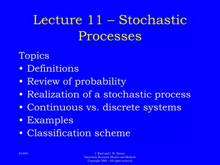
1. Lecture 11 – Stochastic Processes • Topics • Definitions • Review of probability • Realization of a stochastic process • Continuous vs. discrete systems • Examples • Classification scheme J. Bard and J. W. Barnes Operations Research Models and Methods Copyright 2004 - All rights reserved

2. Basic Definitions Stochastic process: System that changes over time in an uncertain manner State: Snapshot of the system at some fixed point in time Transition: Movement from one state to another • Examples • Automated teller machine (ATM) • Printed circuit board assembly operation • Runway activity at airport

3. Elements of Probability Theory Experiment: Any situation where the outcome is uncertain. Sample Space,S:All possible outcomes of an experiment (we will call it “state space”). Event:Any collection of outcomes (points) in the sample space. A collection of events E1, E2,…,En is said to be mutually exclusive if EiEj =  for all i ≠ j = 1,…,n. Random Variable: Function or procedure that assigns a real number to each outcome in the sample space. Cumulative Distribution Function (CDF),F(·): Probability distribution function for the random variable X such that F(a) = Pr{X ≤ a}.

4. Time: Either continuous or discrete parameter. Model Components (continued) State: Describes the attributes of a system at some point in time. s = (s1, s2, . . . , sv); for ATM example s = (n) Convenient to assign a unique nonnegative integer index to each possible value of the state vector. We call this X and require that for each sX. For ATM example, X = n. In general, Xt is a random variable.

5. Transition: Caused by an event and results in movement from one state to another. For ATM example, Activity: Takes some amount of time – duration. Culminates in an event. For ATM example  service completion. Stochastic Process: A collection of random variables {Xt}, where t T = {0, 1, 2, . . .}.

6. Markovian Property Given that the present state is known, the conditional probability of the next state is independent of the states prior to the present state. Present state at time t is i: Xt = i Next state at time t + 1 is j: Xt+1 = j Conditional Probability Statement of Markovian Property: Pr{Xt+1= j | X0 = k0, X1 = k1,…,Xt = i} = Pr{Xt+1= j | Xt = i}   for t = 0, 1,…, and all possible sequences i, j, k0, k1, . . . , kt–1.

7. Number in system, n (no transient response) Realization of the Process Deterministic Process

8. Number in system, n Realization of the Process (continued) Stochastic Process

9. Pure Death Process; e.g., Delivery of a truckload of parcels Birth-Death Process; e.g., Repair shop for taxi company Birth and Death Processes Pure Birth Process; e.g., Hurricanes

10. Queueing Systems Queue Discipline: Order in which customers are served; FIFO, LIFO, Random, Priority Five Field Notation: Arrival distribution / Service distribution / Number of servers / Maximum number in the system / Number in the calling population

11. Queueing Notation Distributions (interarrival and service times) M = Exponential D = Constant time Ek = Erlang GI = General independent (arrivals only) G = General Parameters s = number of servers K = Maximum number in system N = Size of calling population

12. Finite queue: e.g., Airline reservation system (M/M/s/K) a. Customer arrives but then leaves b. No more arrivals after K Characteristics of Queues Infinite queue: e.g., Mail order company (GI/G/s)

13. Characteristics of Queues (continued) Finite input source: e.g., Repair shop for trucking firm (N vehicles) with s service bays and limited capacity parking lot (K – s spaces). Each repair takes 1 day (GI/D/s/K/N). In this diagram N = K so we have GI/D/s/K/K system.

14. Examples of Stochastic Processes Service Completion Triggers an Arrival: e.g., multistage assembly process with single worker, no queue. state = 0, worker is idle state = k, worker is performing operation k = 1, . . . , 5

15. s1 = number of parts in system s2 = current operation being performed s = (s1, s2) where { d d 3 d 3 3 d d d 2 2 2 d d d 1 1 1 Examples (continued) Multistage assembly process with single worker with queue. (Assume 3 stages only) … 1,3 2,3 3,3 a a Assume k = 1, 2, 3 … 1,2 2,2 3,2 a a … 0,0 1,1 2,1 3,1 a a a

16. 0 if server i is idle i = 1, 2 1 if server i is busy s = (s1, s2 , s3) where si = { s3 =number in queue State-transition network Queueing Model with Two Servers, One Operation

17. si = { 0 if server i is idle 1 if server i is busy for i = 1, 2, 3 Series System with No Queues

18. State-transition matrix P = Transitions for Markov Processes Exponential interarrival and service times (M/M/s) State space: S = {1, 2, . . .} Probability of going from state i to state j in one move: pij Theoretical requirements: 0 pij 1, jpij = 1, i = 1,…,m

19. State-transition network Single Channel Queue – Two Kinds of Service Bank teller: normal service (d), travelers checks (c), idle (i) Let p = portion of customers who buy checks after normal service s1 = number in system s2 = status of teller, where s2Î {i, d, c}

20. State-transition network a = arrival s1 = service completion from state 1 s2 = service completion from state 2 Part Processing with Rework Consider a machining operation in which there is a 0.4 probability that upon completion, a processed part will not be within tolerance. Machine is in one of three states: 0 = idle, 1 = working on part for first time, 2 = reworking part.

21. Markov Chains • A discrete state space • Markovian property for transitions • One-step transition probabilities, pij, remain constant over time (stationary) Example: Game of Craps Roll 2 dice: Win = 7 or 11; Loose = 2, 3, 12; otherwise 4, 5, 6, 8, 9, 10 (called point) and roll again  win if point  loose if 7 otherwise roll again, and so on. (There are other possible bets not include here.)

22. State-Transition Network for Craps

23. Transition Matrix for Game of Craps

24. State-Transition Network for Simple Markov Chain

25. Classification of States Accessible: Possible to go from state i to state j (path exists in the network from i to j). Two states communicate if both are accessible from each other. A system is irreducible if all states communicate. State i is recurrent if the system will return to it after leaving some time in the future. If a state is not recurrent, it is transient.

26. a. Each state visited every 3 iterations b. Each state visited in multiples of 3 iterations Classification of States (continued) A state is periodic if it can only return to itself after a fixed number of transitions greater than 1 (or multiple of a fixed number). A state that is not periodic is aperiodic.

27. Classification of States (continued) An absorbingstate is one that locks in the system once it enters. This diagram might represent the wealth of a gambler who begins with $2 and makes a series of wagers for $1 each. Let ai be the event of winning in state i and dithe event of losing in state i. There are two absorbing states: 0 and 4.

28. Classification of States (continued) Class: set of states that communicate with each other. A class is either all recurrent or all transient and may be either all periodic or aperiodic. States in a transient class communicate only with each other so no arcs enter any of the corresponding nodes in the network diagram from outside the class. Arcs may leave, though, passing from a node in the class to one outside.

29. Illustration of Concepts Example 1 Every pair of states communicates, forming a single recurrent class; however, the states are not periodic. Thus the stochastic process is aperiodic and irreducible.

30. Illustration of Concepts Example 2 States 0 and 1 communicate and for a recurrent class. States 3 and 4 form separate transient classes. State 2 is an absorbing state and forms a recurrent class.

31. Illustration of Concepts Example 3 Every state communicates with every other state, so we have irreducible stochastic process. Periodic? Yes, so Markov chain is irreducible and periodic.

32. What you Should know about Stochastic Processes • What a state is • What a realization is (stationary vs. transient) • What the difference is between a continuous and discrete-time system • What the common applications are • What a state-transition matrix is • How systems are classified