Download
1 / 68
760 likes | 1.68k Views
© 2007 Thomson South-Western Short-Run Aggregate Fluctuations Economic activity fluctuates from year to year. In most years production of goods and services rises. On average over the past 50 years, production in the U.S. economy has grown by about 3 percent per year.

E N D
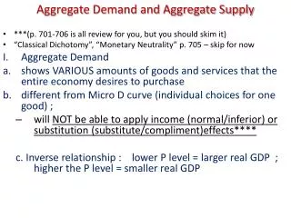
Short-Run Aggregate Fluctuations • Economic activity fluctuates from year to year. • In most years production of goods and services rises. • On average over the past 50 years, production in the U.S. economy has grown by about 3 percent per year. • In some years normal growth does not occur, indicating a recession.
Aggregate Demand and Aggregate Supply • What causes short-run fluctuations in economic activity? • What can public policy do to prevent periods of falling incomes and rising unemployment rate? • When recessions (景氣衰退)and depressions (經濟蕭條)occur, how can policymakers reduce their length and severity?
Aggregate Demand and Aggregate Supply • Our focus is on the economy’s short-run fluctuations(短期波動) around its long-run trend(長期趨勢). • This chapter introduces the aggregate demand curve and the aggregate supply curve.
Short-Run Economic Fluctuations • A recession is a period of slowdown in economic growth or declining real incomes, and rising unemployment rate. • A depression is a severe recession.
THREE KEY FACTS ABOUT ECONOMIC FLUCTUATIONS • Economic fluctuations are irregular and not completely predictable. • Aggregate fluctuations in the economy are often called the business cycle. • These fluctuations do not follow regular or easily predictable patterns. • The longest period in U.S. history without a recession was the economic expansion from 1991 to 2001.
Real GDP A Look At Short-Run Economic Fluctuations (a) Real GDP Billions of 2000 Dollars $10,000 9,000 8,000 7,000 6,000 5,000 4,000 3,000 2,000 196 5 197 0 197 5 198 0 198 5 199 0 199 5 200 0 2005
THREE KEY FACTS ABOUT ECONOMIC FLUCTUATIONS • Most macroeconomic variables move together. • Most macroeconomic variables that measure some type of income, spending, or production fluctuate closely together. • Although many macroeconomic variables fluctuate together, they fluctuate by different amounts. • Aggregate fluctuations in the economy are often called the business cycle. • Consumption varies smoothly over business cycles, while investment varies greatly over business cycles.
Investment Spending A Look At Short-Run Economic Fluctuations (b) Investment Spending Billions of 2000 Dollars $1,500 1,000 500 0 196 5 197 0 197 5 198 0 198 5 199 0 199 5 200 0 2005
THREE KEY FACTS ABOUT ECONOMIC FLUCTUATIONS • As output falls, unemployment rises. • Changes in real GDP are inversely related to changes in the unemployment rate. • During times of recession, unemployment rises substantially. • When the recession ends and real GDP starts to expand, the unemployment rate gradually declines.
Unemployment Rate A Look At Short-Run Economic Fluctuations (c) Unemployment Rate Percent of Labor Force 12% 10 8 6 4 2 196 5 197 0 197 5 198 0 198 5 199 0 199 5 200 0 2005
EXPLAINING SHORT-RUN ECONOMIC FLUCTUATIONS • The Assumptions of Classical Economics • Most economists believe that classical theory describes the world in the long run but not in the short run. • Changes in the money supply affect nominal variables but not real variables in the long run. • The assumption of monetary neutrality is not appropriate when studying year-to-year changes in the economy.
EXPLAINING SHORT-RUN ECONOMIC FLUCTUATIONS • Most economists believe that classical theory describes the world in the long run but not in the short run. • In the short run, real and nominal variables are highly intertwinded, and changes in the money supply can temporarily push real GDP away from its long run trend. • Our new model focuses on how real and nominal variables interact.
EXPLAINING SHORT-RUN ECONOMIC FLUCTUATIONS • If the quantity of money in the economy were to double, prices would double and so would incomes. Real variables would remain constant. • However, these changes will not occur instantaneously. It takes time for prices and incomes to change, and in the meantime, there can be real effects.
The Model of Aggregate Demand and Aggregate Supply • Two variables are used to develop a model to analyze the short-run fluctuations. • The economy’s output of goods and services measured by real GDP. • The average level of prices measured by the CPI or the GDP deflator.
Business cycle Economic activity Time The Model of Aggregate Demand and Aggregate Supply • Economist use the model of aggregate demand (總合需求)and aggregate supply(總合供給)to explain short-run fluctuations in economic activity around its long-run trend.
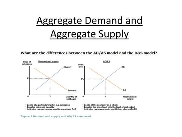
The Model of Aggregate Demand and Aggregate Supply • The aggregate demand curve(總合需求曲線)shows the quantity of goods and services that households, firms, and the government want to buy at each price level. • The aggregate supply curve(總合供給曲線)shows the quantity of goods and services that firms choose to produce and sell at each price level.
THE AGGREGATE-DEMAND CURVE • Why does a change in price level move the quantity of goods and services demanded in the opposite direction? • To answer it, recall that GDP (Y) is the sum of consumption (C), Investment (I), government (G), and net exports (NX): Y = C + I + G + NX
P P2 1. A decrease Aggregate in the price demand level . . . Y Y2 2. . . . increases the quantity of goods and services demanded. The Aggregate-Demand Curve Price Level Quantity of 0 Output
Why the Aggregate-Demand Curve Is Downward Sloping • The Price Level and Consumption: The Wealth Effect(財富效果) • The Price Level and Investment: The Interest Rate Effect(利率效果) • The Price Level and Net Exports: The Exchange Rate Effect(匯率效果)
Why the Aggregate-Demand Curve Is Downward Sloping • The Price Level and Consumption: The Wealth Effect(The least important factor) • A lower price level raises the real value of money and makes consumers wealthier, which encourages them to spend more. • This increase in consumer spending means larger quantities of goods and services demanded.
Why the Aggregate-Demand Curve Is Downward Sloping • The Price Level and Investment: The Interest Rate Effect (The most important factor) • The lower the price level, the less money households need to hold to buy goods and services they want. • When the price level falls, households try to reduce their holding of money either by buying interest-bearing bonds or by depositing excess money in saving accounts. • In either case, they drive down interest rate. • A lower interest rate encourages firms to borrow more to invest in new plant and equipment, and also encourages households to borrow more to invest in new housing. • Thus, a lower interest rate increases the quantity of goods and services demanded.
Why the Aggregate-Demand Curve Is Downward Sloping • The Price Level and Net Exports: The Exchange Rate Effect • A lower price level in Taiwan causes the Taiwan interest rates to fall. In response to the lower Taiwan interest rate, some Taiwan investors will seek higher returns by investing abroad. This will increase the supply of N.T. dollars in the foreign currency exchange market. • It will cause N.T. dollars to depreciate relative to the foreign currency, and hence stimulates Taiwan net exports. • The increase in net export spending means a larger quantity of goods and services demanded.
Why the Aggregate-Demand Curve Might Shift • The downward slope of the aggregate-demand curve shows that a fall in the price level raises the overall quantity of goods and services demanded. • Many other factors, however, affect the quantity of goods and services demanded at any given price level. • When one of these other factors changes, the aggregate demand curve shifts.
Why the Aggregate-Demand Curve Might Shift • Shifts might arise from changes in: • Consumption • Investment in economic boom and recession • Government Purchases • Tax policy • Net Exports due to boom and recession in world markets
D2 Y2 Shifts in the Aggregate Demand Curve Price Level P1 Aggregate demand, D1 0 Y1 Quantity of Output
THE AGGREGATESUPPLY CURVE • Classical macroeconomics predicts the quantity of goods and services produced by an economy in the long run. • In the long run, the aggregate-supply curve is vertical because the price level does not affect long run determinants of real GDP. • The long-run level of output is called the natural rate of output since it shows what the economy produces when unemployment is at its natural rate. • In the short run, the aggregate-supply curve is upward sloping.
THE AGGREGATESUPPLY CURVE • In the long run, an economy’s production of goods and services depends on its supplies of labor, capital, and natural resources and on the available technology used to turn these factors of production into goods and services. • The price level does not affect these variables in the long run. • The long-run aggregate supply represents the classical dichotomy and money neutrality.
P P2 2. . . . does not affect 1. A change the quantity of goods in the price and services supplied level . . . in the long run. The Long-Run Aggregate-Supply Curve is Vertical Price Level Long-run aggregate supply Quantity of 0 Natural rate Output of output
THE AGGREGATE-SUPPLY CURVE • The long-run aggregate-supply curve is vertical at the natural rate of output(自然產出率), which is the production of goods and services that an economy achieves in the long run when unemployment is at its natural rate. • This level of production is also referred to as potential output or full-employment output(充分就業產出水準). • The natural rate of output is level of output towards which the economy gravitates in the long run.
Why the Long-Run Aggregate-Supply Curve Might Shift • Any change in the economy that alters the natural rate of output shifts the long-run aggregate-supply curve. • The shifts may be categorized according to the various factors in the classical model that affect output.
Why the Long-Run Aggregate-Supply Curve Might Shift • Shifts might arise from changes in: • Labor (increases in immigration, increases in minimum wage rate) • Accumulation in physical and human capital • Natural Resources (oil shocks) • Technological Knowledge (Trade openness)
2. . . . and growth in the money supply shifts aggregate demand . . . LRAS LRAS 1990 2000 1. In the long run, technological progress shifts long-run aggregate P 2000 supply . . . 4. . . . and ongoing inflation. P 1990 Aggregate Demand, AD 2000 AD 1990 Y Y 1990 2000 3. . . . leading to growth in output . . . Long-Run Growth and Inflation Long-run aggregate supply, LRAS 1980 Price Level P 1980 AD 1980 Quantity of 0 Y 1980 Output
Using Aggregate Demand and Aggregate Supply to Depict Long-Run Growth and Inflation • The most important forces that govern the economy in the long run are technology and monetary policy. • Short-run fluctuations in output and the price level should be viewed as deviations from the continuing long-run trends of output growth and inflation.
Why the Aggregate-Supply Curve Slopes Upward in the Short Run • In the short run, an increase in the overall level of prices in the economy tends to raise the quantity of goods and services supplied. • A decrease in the level of prices tends to reduce the quantity of goods and services supplied. • As a result, the short-run aggregate-supply curve is upward sloping.
P P2 2. . . . reduces the quantity 1. A decrease of goods and services in the price supplied in the short run. level . . . Y2 Y The Short-Run Aggregate-Supply Curve is Upward Sloping Price Level Short-run aggregate Supply (S-RAS) Quantity of 0 Output
Why the Aggregate-Supply Curve Slopes Upward in the Short Run • Three Theories: • The Sticky-Wage Theory (薪資僵固理論) • The Sticky-Price Theory(價格僵固理論) • The Misperceptions Theory(對價格變動錯誤解讀理論)
Why the Aggregate-Supply Curve Slopes Upward in the Short Run • The Sticky-Wage Theory • Nominal wages are slow to adjust to changing economic conditions, or are “sticky” in the short run. • When nominal wages are based on the expected prices and do not respond immediately when the actual price level turns out to be different from what was expected. • This stickiness gives firms an incentive to produce less (more) when the price level turns out lower (higher) than expected. • The slow can be attributed to long-term contract between workers and firms. • This induces firms to reduce the quantity of goods and services supplied.
Why the Aggregate-Supply Curve Slopes Upward in the Short Run • The Sticky-Price Theory • Prices of some goods and services adjust sluggishly in response to changing economic conditions. • This slow adjustment of prices occurs in part because there are costs to adjusting prices, called menu costs. • An unexpected fall in the price level leaves some firms with higher-than-desired prices. For a variety of reasons, they may not want to or be able to change prices immediately. • This depresses sales, which induces firms to reduce the quantity of goods and services they produce.
Why the Aggregate-Supply Curve Slopes Upward in the Short Run • The Misperceptions Theory • Changes in the overall price level temporarily mislead suppliers about what is happening in the markets in which they sell their output. • A lower price level causes misperceptions about relative prices. • These misperceptions induce suppliers to decrease the quantity of goods and services supplied.
Quantity of output supplied Natural rate of output Actual price level Expected price level = a - + Why the Aggregate-Supply Curve Slopes Upward in the Short Run • All three theories suggest that output deviates in the short run from the natural rate when the actual price level deviates from the price level that people had expected to prevail.
S-RAS Equilibrium price level AD Equilibrium output The Determination of Short-Run Equilibrium Price Level Quantity of 0 Output
Short-run aggregate supply A Equilibrium price Aggregate demand Natural rate of output The Long-Run Equilibrium Price Level Long-run aggregate supply Quantity of 0 Output
In long-run equilibrium, • Short-run equilibrium co-inside with long-run equilibrium at point A. • At point A, actual inflation rate equals expect inflation rate . • In long-run equilibrium, the equilibrium quantity of output equals the natural rate of output.
When short-run equilibrium differs from long-run equilibrium