Download
1 / 45
490 likes | 1.24k Views
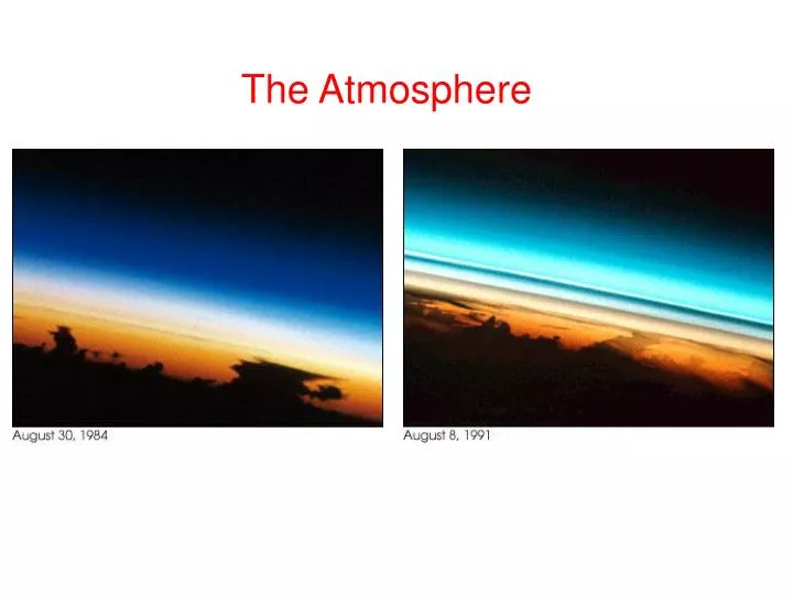
The Atmosphere. Atmospheric structure. Atmospheric layers defined by changes in temperature Troposphere – contains 75% of atmospheric gases; temperature decreases with height Tropopause – boundary between troposphere and stratosphere; location of the jet stream

E N D
Atmospheric structure • Atmospheric layers defined by changes in temperature • Troposphere – contains 75% of atmospheric gases; temperature decreases with height • Tropopause – boundary between troposphere and stratosphere; location of the jet stream • Tropopause altitude varies from ~8 km (Poles) to ~17 km (Tropics) • Stratosphere – contains the ozone layer, which causes the temperature to increase • Thermosphere: highly energetic solar radiation (UV, X-rays) absorbed by residual atmospheric gases
Tropopause altitude Cumulonimbus cloud over Africa (photo from International Space Station) • Tropopause altitude is dependent on latitude – it is highest in the tropics where convection is strong • The tropopause is not a ‘hard’ boundary – it can be defined thermally, dynamically or chemically
Planetary boundary layer (PBL) • PBL height • 300 m – 3 km • Influenced by convection • Varies diurnally • The PBL is the lowest part of the atmosphere – directly influenced by contact with the planetary surface • Responds to changes in surface forcing rapidly (hours) • Quantities such as flow velocity, temperature, moisture show rapid variations (turbulence) and vertical mixing is strong • PBL winds are affected by surface drag, as opposed to winds in the ‘free troposphere’ above which are determined by pressure gradients
Atmospheric pressure Hypsometric equation h = layer thickness (m) R = ideal gas constant (8.314 J K-1 mol-1) T = temperature (K) g = gravitational acceleration (9.81 m s-2) P = pressure (Pa) • Atmospheric pressure is the weight of the gases surrounding the earth. It is a function of height, density and gravity. • Energy (motion) at the molecular level creates atmospheric pressure and prevents the atmosphere from collapsing on itself • At ground level it is recorded as 101.32 kilopascals (kPa) ; equal to 14.7 lbs. per sq. inch or 760 mm Hg (also 1 atmosphere, 1 bar, 1000 millibars etc.) • Atmospheric pressure decreases exponentially with altitude: at 18,000 ft. (~6 km) it is halved and at 33,000 ft., (~11 km) quartered • Note that in water atmospheric pressure doubles at at a depth of 33 ft
The Standard Atmosphere • Standard (or model) atmospheres facilitate comparison of radiative transfer models • They represent ‘typical’ atmospheric conditions for a particular region/season • Used whenever an actual sounding (measurement of the atmospheric state) is not available • At least 7 standard model atmospheres are in common use: tropical (warm, humid, high tropopause), midlatitude summer, midlatitude winter, subarctic summer, subarctic winter, arctic summer and arctic winter (cold, dry, low tropopause)
Atmospheric composition Composition of dry atmosphere, by volume Nitrogen (N2) 78% (780,840 ppmv) Oxygen (O2) 21% (209,460 ppmv) Argon (Ar) 0.93% (9340 ppmv) Carbon dioxide (CO2) 0.04% (383 ppmv) Neon (Ne) 0.002% Helium (He) 0.0005% Methane (CH4) 0.0001% Krypton (Kr) Hydrogen (H2) Nitrous oxide (N2O) Ozone (O3) 0-0.07 ppmv Water vapor (H2O) 1-4% at surface ppmv = parts per million by volume = volume mixing ratio
Trace constituents Some atmospheric trace gases of environmental significance
CO2 concentrations Measurements of atmospheric carbon dioxide at Mauna Loa Observatory, Hawaii (Keeling curve)
The Ozone Layer • The stratospheric ozone layer is a consequence of molecular photodissociation • UV-C radiation dissociates molecular oxygen: • O2 + hv (λ < 0.2423 µm) O + O • The large amount of oxygen in the atmospheric column absorbs most solar radiation at λ < 0.24 µm by this mechanism • The free oxygen atoms from the above reaction then combine with other O2 molecules to produce ozone: • O + O2 O3 • Ozone is then dissociated by UV radiation: • O3 + hv (λ < 0.32 µm) O + O2 • Ozone is also destroyed by this reaction: • O3 + O O2 + O2 The Chapman Reactions
The Ozone Layer • Fortunately for life on Earth, ozone absorbs strongly between 0.2 and 0.31 µm via electronic transitions – removing most UV-B and UV-C not absorbed by O2 • UV-A radiation (λ > 0.32 µm) is transmitted to the lower atmosphere • Plus a small fraction of UV-B (0.31-0.32 µm) – responsible for sunburn • Widening of this UV-B window (due to ozone depletion) would have serious impacts on life • Absorption of solar radiation by ozone also locally warms the atmosphere to a much higher temperature than would be possible if ozone was absent – hence the increase in T in the stratosphere • Hence in an atmosphere without free oxygen, and hence without ozone, the temperature would decrease with height until the thermosphere. There would be no stratosphere, and weather would be vastly different...
The Ozone Layer • Most of the ozone production occurs in the tropical upper stratosphere and mesosphere, but the ozone maximum occurs at mid-latitudes
Ozone hole • Ozone destruction peaks in the Spring, as UV radiation returns to the polar regions • Catalyzed by the presence of CFC compounds (which supply chlorine), and by polar stratospheric clouds (PSCs) at very cold temperatures Antarctic ozone hole on Sept 11, 2005 Observed by Ozone Monitoring Instrument (OMI)
Ozone is not just in the stratosphere.. • The UV-A radiation that reaches the troposphere is a key player in tropospheric chemistry • Photochemical reactions involving unburned fuel vapors (organic molecules) and nitrogen oxides (produced at high temperatures in car engines) produce ozone in surface air (tropospheric ozone) • Ozone is good in the stratosphere, but a hazard in the troposphere (it is a strong oxidant that attacks organic substances, such as our lungs) • Ozone is a major ingredient of photochemical smog λ < 0.4 µm Los Angeles: sunshine (UV) + cars + trapped air = smog
Adiabatic cooling • As an air parcel rises, it will adiabatically expand and cool • Adiabatic: temperature changes solely due to expansion or compression (change in molecular energy), no heat is added to or removed from the parcel
Atmospheric stability Dry air – no condensation Dry adiabatic lapse rate = ~10ºC km-1 Atmospheric stability is assessed by comparing the environmental lapse rate with the adiabatic lapse rate
Atmospheric stability Moist air – condensation provides heat Moist adiabatic lapse rate = ~6.5ºC km-1
Atmospheric stability Dry air Lapse rate < adiabatic lapse rate Lapse rate > adiabatic lapse rate
Atmospheric stability Same lapse rate > moist adiabatic lapse rate (Thunderstorm) Lapse rate < dry adiabatic lapse rate
Water in the atmosphere • There are about 13 million million tons of water vapor in the atmosphere (~0.33% by weight) • In gas phase – absorbs longwave radiation and stores latent heat • Responsible for ~70% of atmospheric absorption of radiation • In liquid and solid phase – reflects and absorbs solar radiation
Temperature inversions A temperature inversion occurs when a layer of cool air is trapped at ground level by an overlying layer of warm air, which can also trap pollutants. Many factors can lead to an inversion layer, such as temperatures that remain below freezing during the day, nighttime temperatures in the low teens to single digits, clear skies at night, and low wind levels.
Pollution trapping Salt Lake valley, Utah
Radiosondes • A radiosonde is a package of instruments mounted on a weather balloon that measures various atmospheric parameters and transmits the data to a fixed receiver (sometimes called a rawinsonde if wind speed is measured) • Measured parameters usually include: pressure, altitude, latitude/longitude, temperature, relative humidity and wind speed/direction • The maximum altitude to which the helium or hydrogen-filled balloon ascends is determined by the diameter and thickness of the balloon • At some pressure, the balloon expands to the extent that it bursts (maybe ~20 km) – the instrument is usually not recovered • Worldwide there are more than 800 radiosonde launch sites • Radiosonde launches usually occur at 0000 and 1200 UTC • ‘Snapshot’ of the atmosphere for modeling and forecasting
Radiosonde soundings • INFORMATION OBTAINED FROM RAOB SOUNDINGS: • The radiosonde transmits temperature and relative humidity data at each pressure level. Winds aloft are determined from the precision radar tracking of the instrument package. The altitudes of these levels are calculated using an equation (the hypsometric equation) that relates the vertical height of a layer to the mean layer temperature, the humidity of the layer and the air pressure at top and bottom of the layer. Significant levels where the vertical profiles of the temperature or the dew point undergo a change are determined from the sounding. The height of the troposphere and stability indices are calculated. • A plot of the vertical variations of observed weather elements made above a station is called a sounding. • The plots of the air temperature, dew point and wind information as functions of pressure are generally made on a specially prepared thermodynamic diagram.
Saturation mixing ratio Stüve diagrams isobars • A Stüve diagram is one of four thermodynamic diagrams used in weather data analysis and forecasting • Radiosonde temperature and dew point data may be plotted on these diagrams to assess convective stability. Wind barbs may be plotted next to the diagram to indicate the vertical wind profile. Moist adiabatic lapse rate Dry adiabatic lapse rate isotherms • Straight lines show the 3 primary variables: pressure, temperature and potential temperature • Isotherms are straight and vertical, isobars are straight and horizontal • Dry adiabats are straight and inclined 45º to the left; moist adiabats are curved • Dew point: temperature to which air must be cooled (at constant pressure) for water vapor to condense to water (i.e. for clouds to form)
Skew T - log P diagrams Dry adiabats Skew T-log p--Example isobars isotherms moist adiabatic lapse rate Saturation mixing ratio
Wind barbs 1 knot = 0.514 m s-1
Radiosonde soundings Currently, 70 RAOB stations are distributed across the continental USA http://weather.uwyo.edu/upperair/sounding.html
Radiosonde sounding – Green Bay Tropopause Stüve
Ideal Gas Law • The equation of state of an ideal gas – most gases are assumed to be ideal • P = pressure (Pa), V = volume taken up by gas (m3), n = number of moles, R = gas constant (8.314 J mol-1 K-1), T = temperature (K) • k = Boltzmann constant (1.38×10⁻²³ J K-1), N = number of molecules, NA= Avogadro constant (6.022×10²³ molecules mol-1) • Neglects molecular size and intermolecular attractions • States that volume changes are inversely related to pressure changes, and linearly related to temperature changes • Decrease pressure at constant volume = temperature must decrease (adiabatic cooling)
Ideal gases • Standard temperature and pressure (STP): varies with organization • Usually P = 101.325 kPa (1 atm) and T = 273.15 K (0ºC) • Sometimes P = 101.325 kPa and T = 293.15 K (20ºC) • At STP (101.325 kPa, 273.15 K) each cm3 of an ideal gas (e.g., air) contains 2.69×10¹⁹ molecules (or 2.69×1025 m-3) • This number is the Loschmidt constant and can be derived by rearranging the ideal gas law equation: • At higher altitudes, pressure is lower and the number density of molecules is lower • Mean molar mass of air = 0.02897 kg mol-1 (air is mostly N2)
Quantification of gas abundances • The concentration (c) of a gas is the amount of gas in a volume of air: • ‘Amount’ could be mass, number of molecules, or number of moles • Common units are micrograms per m3(µg m-3) or molecules per m3 – the latter is the number density of the gas. Partial pressures of gases are also sometimes used. • We also define the mixing ratio of a gas: • ‘Amount’ could be volume, mass, number of molecules, or number of moles. In atmospheric chemistry, it is usually volume. • Example of a mixing ratio in parts per million by volume (ppmv; sometimes just written as ppm):
Quantification of gas abundances • Smaller mixing ratios are given in parts per billion (ppbv) or parts per trillion (pptv): • Mixing ratios can also be expressed by mass; the default is usually volume (i.e. ppb usually implies ppbv) • For an ideal gas the volume mixing ratio is equal to the molar mixing ratio (xm) or mole fraction (this is the SI unit for mixing ratios): • So micromole per mole, nanomole per mole and picomole per mole are equivalent to ppmv, ppbv and pptv, respectively • Remember the conversion factor! (ppmv = 106, ppbv = 109, pptv = 1012 etc.) • MIXING RATIOS ARE INDEPENDENT OF TEMPERATURE AND PRESSURE • Concentrations, however, are not (they change when air is transported)
Vertical profile of ozone Vertical profiles of atmospheric constituents look different depending on the abundance units used
Conversion of abundance units • For a gas i, the conversion between number density cn (in molecules cm-3) and mass concentration cm (in grams cm-3) is: • Mi = molecular weight of species i (grams mol-1) • NA = Avogadro constant (6.022×10²³ molecules mol-1) • Hence this conversion depends on the molecular mass of the gas • Conversion from number density cn (in molecules cm-3) to volume mixing ratio: • V = molar volume (cm3) for the pressure and temperature at which the number density was measured • At STP, V = 22414 cm3 mole-1. For arbitrary T and P, use the ideal gas law:
Abundance units for trace gases Spectroscopic remote sensing techniques give results in number density, not mixing ratios (recall Beer’s Law)
Unit conversion example • The Hong Kong Air Quality Objective for ozone is 240 µg m-3 • The U.S. National Ambient Air Quality Standard for ozone is 120 ppb • Which standard is stricter at the same temperature (25ºC) and pressure (1 atm)? • REMEMBER TO USE CONSISTENT (SI) UNITS • We need to convert 240 µg m-3 to a mixing ratio in ppb • On the right hand side we have: • So we need cm in g m-3 • Which is 240×10-6 g m-3 • This gives xv = 1.22×10-7 × 109 nanomoles per mole = 122 ppb
Column density • Another way of expressing the abundance of a gas is as column density (Sn), which is the integral of the number density along a path in the atmosphere • The unit of column density is molecules cm-2 • The integral of the mass concentration is the mass column density Sm (typical units are µg cm-2) • Usually the path is the entire atmosphere from the surface to infinity, called the total column, giving the total (vertical) atmospheric column density, V:
Dobson Units • A Dobson Unit [DU] is a unit of column density used in ozone research, and in measurements of SO2 • Named after G.M.B. Dobson, one of the first scientists to investigate atmospheric ozone (~1920 – 1960) • The illustration shows a column of air over Labrador, Canada. The total amount of ozone in this column can be conveniently expressed in Dobson Units (as opposed to typical column density units). • If all the ozone in this column were to be compressed to STP (0ºC, 1 atm) and spread out evenly over the area, it would form a slab ~3 mm thick • 1 Dobson Unit (DU) is defined to be 0.01 mm thickness of gas at STP; the ozone layer represented above is then ~300 DU (NB. 1 DU also = 1 milli atm cm)
Dobson Units • So 1 DU is defined as a 0.01 mm thickness of gas at STP • We know that at STP (101.325 kPa, 273.15 K) each cm3 of an ideal gas (e.g., air, ozone, SO2) contains 2.69×10¹⁹ molecules (or 2.69×1025 m-3) • So a 0.01 mm thickness of an ideal gas contains: • 2.69×10¹⁹ molecules cm-3 × 0.001 cm = 2.69×10¹⁶ molecules cm-2 =1 DU • Using this fact, we can convert column density in Dobson Units to mass of gas, using the cross-sectional area of the measured column at the surface • For satellite measurements, the latter is represented by the ‘footprint’ of the satellite sensor on the Earth’s surface
The Ozone Layer • Map shows total column ozone in DU