Download
1 / 62
660 likes | 928 Views
Algebraic Geometric Coding Theory presented by. Jake Hustad. John Hanson. Berit Rollay. Nick Bremer. Tyler Stelzer. Robert Coulson. Contents. Review of Codes The Performance Parameters Reed-Solomon Code Finite Fields/Algebraic Closure The Projective Plane

E N D
Algebraic Geometric Coding Theory presented by Jake Hustad John Hanson Berit Rollay Nick Bremer Tyler Stelzer Robert Coulson
Contents • Review of Codes • The Performance Parameters • Reed-Solomon Code • Finite Fields/Algebraic Closure • The Projective Plane • Bezout’s Theorem • Frobenius Maps • Nonsingularity and Genus • Goppa’s Construction • Conclusion
Review of Codes Jake Hustad
Introduction • Basic Overview of Coding Theory • Coding theory is the branch of mathematics concerned with • transmitting data across noisy channels and recovering the • message. Coding theory is about making messages easy • to read and finding efficient ways of encoding data.
What is a Code? Here is the formal definition of a code: A code C over an alphabet is simply a subset of An = A x…x A(n copies). Where is usually a finite field.
Objectives for efficient codes: • Detection and correction of errors due to noise • Efficient transmission of data • Easy encoding and decoding schemes
The Ideal Code • Ideally, we would like a code that is capable of correcting all errors due to noise. In general, the more errors that a code needs to correct per message digit, the less efficient the transmission and also the more complicated the encoding and decoding schemes.
The Performance Parameters • “n” is the total number of available symbols for a code word. • “k” is the number of information symbols in a given code word. “k” is the size of the code. • “d” is the distance between two code words. This is a Hamming distance.
The Hamming Distance The Hamming distance between two words is the number of places where the digits differ.
Example • u = “111” (Transmitted Code)v = “110” (Received Code)They differ only in the last digit, so the Hamming distance, d(u,v) = 1.
The Hamming Distance • This distance is significant because it gives us an idea of how many errors can be detected. The larger this distance is, the more errors can be detected.
The Minimum Distance The minimum distance is the smallest Hamming distance between any two possible code words.
The Minimum Distance • Suppose that the minimum distance for the coding function is 3. Then, given any codeword, at least 3 places in it have to be changed before it gets converted into another codeword. In other words, if up to 2 errors occur, the resulting word will not be a codeword, and we detect the occurrence of errors.
The Minimum Distance • Fact: If the minimum distance between code words is d, then up to d – 1 errors can be detected.
Reed-Solomon Codes A Case Study John Hanson
Definitions Fq ~ field with q elements Lr := { f Fq[x] | deg(f) r } {0} r is non-negative note: this is a vector subspace over Fq with dim = r+1 basis = [ 1 x x2 … xr ]
Procedure • Label q-1 nonzero elements of Fq as:1, 2,…, q-1 • Pick a k Z such that 1 k q-1 Then we have:RS(k,q) := { ( f( 1), f( 2),…,f( q-1) )| f Lk-1 }
Notice • RS(k,q) is a subset of := FqxFqx…xFqq-1 copies so this is a code over the alphabet Fq
Summary • Through our research and presentation last semester, we proved that for Reed-Solomon codes: n = q – 1 k = k (which was chosen) d = n – k + 1
Algebraic Geometry Background By Nick Bremer and Berit Rollay
Contents • Finite Fields/Algebraic Closure • Projective Planes • Bezout’s Theorem
A field k is algebraically closed if every non-constant polynomial in k[x] has at least one root. Ex) Algebraically Closed Fields This is not closed under R because i ÏR, but it is closed under C.
Definition: Algebraic Closure Let k be a field. An algebraic closure of k is a field K with k K satisfying: • K is algebraically closed, and • If L is a field such that k L K and L is algebraically closed, then L = K.
Ex) Are Algebraic Closures Unique? It turns out they are. Every field has an unique algebraic closure, up to isomorphism. This theorem allows us to call the algebraic closure of k.
Theorem Let k be an algebraically closed field and let be a polynomial of degree n. Then there exists a non-zero u and (not necessarily distinct) such that: In particular, counting multiplicity, f has exactly n roots in k.
Diophantine Equations A Diophantine Equation is a polynomial with integer or rational coefficients, such as . A useful problem to solve is how many rational solutions does this equation have? In order to answer this question, we need to define points at “infinity.”
Projective Plane Let k be a field. The projective plane is defined as: where if and only if there is some non-zero with , and . a
Projective Plane, con’t To further understand the projective plane, consider the following illustration: The projective plane can be described as all of the lines in R3that pass through the origin. Further, we can say that lines that intersect the plane P shown above represent “real” points, and lines that do not intersect the plane represent points at “infinity.” These terms will be defined in more depth momentarily.
Where the homogenization of f is: Homogenization Let k be a field, a polynomial of degree d, and Cfthe curve associated to f (f(x,y)=0). The projective closure of the curve Cf is:
Example of Homogenization Consider the curve . If we take the Homogenization, we get: Now we are ready to solve the Diophantine Equation.
Any point in the homogenization that is of the form with is called a point at infinity. Remember the Diophantine Equation? Now we can find all solutions to a Diophantine Equation, including solutions that occur at “infinity.” • All other points are called affine points.
Bezout’s Theorem If are polynomials of degrees d and e respectively, then and intersect in at most de points. Further, and intersect in exactly de points of , when points are counted with multiplicity. This is used in a classical proof of algebraic geometry, but we will not go into that at this time.
Points, Divisors and Rational Functions By Tyler Stelzer and Bob Coulson
Frobenius Maps Suppose Fq is a finite field (recall this means that q must be a prime power) and that n >= 1. The Frobenius Automorphism is the map σq,n : Fqn Fqn defined by σq,n(α) = αq, for any α Fqn
Relative and Absolute Frobenius • If q = pr where p is prime and r >= 2, then • the map σq,n is often called the relative Frobenius • the function σp,n if often called the absolute Frobenius
Composing Frobenius with Itself The symbol σjq,n represents the map obtained by composing σq,n with itself j times. For example: σ2q,n (α) = σq,n (σq,n(α)).
Nonsingularity When constructing a code, one of the elements needed is a nonsingular projective plane curve. A projective plane curve, Cf, is nonsingular when no singular points exist on it.
Singular Points • A singular point of Cf is a point (x0,y0) such that f (x0,y0) = 0 and fx(x0,y0) = 0 and fy(x0,y0) = 0. • Or if F(X,Y,Z) is the homogenization of f(x,y), then (X0:Y0:Z0) is a singular point of Cfif the point is on the curve and: • F (X0:Y0:Z0) = Fx (X0:Y0:Z0) = Fy (X0:Y0:Z0) = Fz(X0:Y0:Z0) = 0.
What are f(x,y), fx(x,y) f y(x,y)? • What is f(x,y)? • A singular point of Cf is a point (x0,y0) such that f(x0,y0) = 0 and fx(x0,y0) = 0 and fy(x0,y0) = 0. • f(x,y) k[x,y] where k[x,y] is the set of polynomials having coefficients from k and two variables, x and y. • Example: Let k = Z5 = {0,1,2,3,4}. Then one possible polynomial is: f(x,y) = 2x2y + xy3 + x2 + 2y
What are f(x,y), fx(x,y) f y(x,y)? • What is fx(x,y)? • A singular point of Cf is a point (x0,y0) such that f(x0,y0) = 0 and fx(x0,y0) = 0 and fy(x0,y0) = 0. • fx(x,y) is the partial derivative of f(x,y) with respect to x. • Example: Let f(x,y) = 2x2y + xy3 + x2 + 2y Then fx(x,y) = 4xy + y3 + 2x.
What are K, f(x,y), fx(x,y) f y(x,y)? • What is f y(x,y)? • A singular point of Cf is a point (x0,y0) such that f(x0,y0) = 0 and fx(x0,y0) = 0 and fy(x0,y0) = 0. • fy(x,y) is the partial derivative of f(x,y) with respect to y. • Example: Let f(x,y) = 2x2y + xy3 + x2 + 2y Then fy(x,y) = 2x2 + 3xy2 + 2.
Genus and the Plϋcker Formula • A nonsingular curve can be realized as a torus-like object with one or more holes in R3. This torus has a certain number of holes which is called the topological genus (g). The genus is given by the formula g = (d-1)(d-2)/2 where d is the degree of the polynomial which makes the curve nonsingular. This formula is called the Plϋcker Formula.
Points, Functions, andDivisors on Curves Let k be a field, and let C be the projective plane curve defined by F = 0, where F = F(X,Y,Z) k[X,Y,Z] is a homogenous polynomial. For any field K containing k, we define a K-rational point on C to be a point (X0 : Y0 : Z0) P2(K) such that F(X0,Y0,Z0) = 0. The set of all K-rational points on C is denoted C(K). Elements of C(k) are called points of degree one or simply rational points.
Points, Functions, and Divisors on Curves Let C be a nonsingular projective plane curve. A point of degree n on C over Fqis a set P = {P0,…,Pn-1} of n distinct points in C(Fqn) such that Pi = σiq,n(P0) for i = 1,…, n-1.
Points, Functions, and Divisors on Curves • A divisor D on X, a nonsingular projective plane curve, over Fq is an element of the free abelian group on the set of points on X over Fq. Every divisor is of the form where the nQ are integers and each Q is a point on X. If nQ 0 for all Q, D is effective and D 0. The degree of . The support of D is suppD = {Q | nQ 0}.
Points, Functions, and Divisors on Curves Let F(X,Y,Z) be the polynomial which defines the nonsingular projective plane cure C over the field Fq. The field of rational functions on C is where g/h ~ g`/ h` if and only if gh` - g`h ‹F› Fq[X,Y,Z]. g,h Fq[X,Y,Z] are homogeneous of the same degree
Points, Functions, and Divisors on Curves Let C be a curve defined over Fq and let f := g/h Fq(C). The divisor of f is defined to be div(f) := Σ P – Σ Q, where Σ P is the intersection divisor C Cg and Σ Q is the intersection divisor C Ch.
Points, Functions, and Divisors on Curves Let D be a divisor on the nonsingular projective plane curve C defined over the field Fq. Then the space of rational functions associated to D is L(D) := {f Fq(C) | div(f) + D >= 0} {0}.
Riemann-Roch Theorem Let C be a nonsingular projective plane curve of genus g defined over the field Fq and let D be a divisor on X. Then dim L(D) >= deg D + 1 – g. Further, if deg D > 2g – 2, then dim L(D) = deg D + 1 – g.