Surface characteristics and River routing

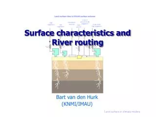
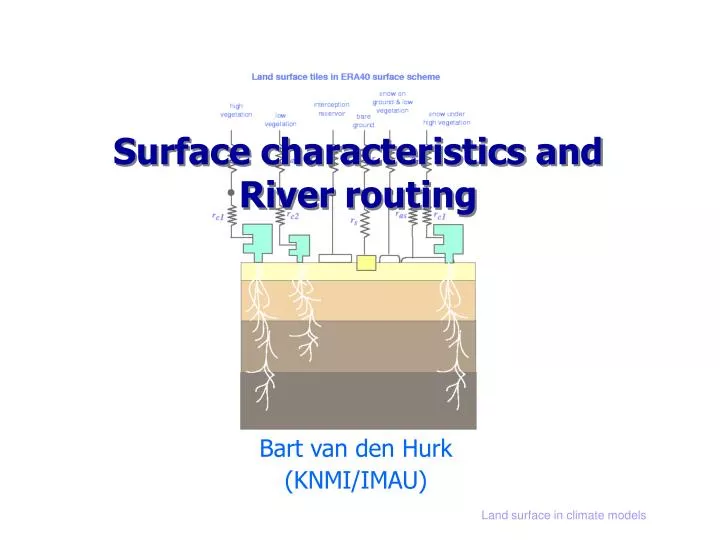
1. Surface characteristics and River routing Bart van den Hurk (KNMI/IMAU) Land surface in climate models

2. Question • Model: • frozen ground does not allow vertical moisture movement • melting snow on frozen ground: runoff • water lost for the warm season • Real world: • some melting water will percolate via large pores or holes • less runoff, more storage • Question: how could we change our parameterization? Land surface in climate models

3. Exercise 1 Bart van den Hurk (KNMI/IMAU) Land surface in climate models

4. Exercise with GSWP2 simulation • GSWP2 = Global Soil Wetness Project • 10 year (1986-1995) after 2.5yrs spin-up • worldwide (~15000 gridpoints) • Forcings: rain, snow, shortwave, longwave, T, q, u, pressure • Model version: H-TESSEL • 6 land tiles (low + high veg, bare, exposed + forest snow, interception) • explicit surface runoff • Van Genuchten soil hydraulics • Jarvis-Stewart canopy resistance • Output • daily prognostic fields (at 0:00 UTC) • daily accumulated fluxes • grouped in ~10 files per month Land surface in climate models

5. o_eva "SubSnow“ # Snow sublimation [kg/m2/s] "ECanop" # Interception evaporation [kg/m2/s] "TVeg" # Vegetation transpiration [kg/m2/s] "ESoil" # Bare soil evaporation [kg/m2/s] "RootMoist" # Root zone soil moisture [kg/m2] "CanopInt" # Canopy interception depth [kg/m2] o_fix "SoilDepth" # Soil depth [m] "M_fielscap" # Field capacity [m3/m3] "M_wilt" # Wilting point [m3/m3] "M_sat" # Saturated soil moisture content [m3/m3] o_gg “SoilMoist" # Soil moisture content [kg/m2] "SoilTemp" # Soil temperature [K] "AvgSurfT" # Avergae skin temperature [K] "Icetemp" # Sea ice temperature [K] "SWE" # Snow mass water eq [kg/m2] "SnowT“ # Snow temperature [K] "Snowdens" # Snow density [kg/m3] o_sub "LSoilMoist" # Diagnostic liquid soil water content [kg/m2] "SoilWet“ # Total soil wetness [-] o_sus "VegT“ # Skin temperature vegetation [K] "BaresoilT" # Skin temperature bare soil [K] "RadT" # Surface radiative temperature [K] "Albedo" # Average albedo [-] o_wat "Rainf" # rainfall rate [kg/m2/s] "Snowf" # snowfall rate [kg/m2/s] "Qs" # total runoff [kq/m2/s] "Qsm“ # snow melt [kg/m2/s] "Qsb“ # base flow [kg/m2/s] "Evap" # evaporation [kg/m2/s] "DelSoilMoist“ # Soil moisture change [kg/m2] "DelIntercept“ # Interception storage change [kg/m2] "DelSWE" # Snow Water Equivalent change [kg/m2] o_cld "SnowDepth" # Snow depth [m] "SnowFrac" # Snow fraction [-] "IceFrac" # Ice covered gridbox fraction [-] "Fdepth“ # Frozen soil depth [m] "Tdepth" # Depth to soil thaw [m] "SAlbedo“ # Snow albedo [-] o_efl "Qle“ # Average latent heat flux [W/m2] "Qh" # Average sensible heat flux [W/m2] "Qg" # Average soil heat flux [W/m2] "Qf" # Average soil fusion flux [W/m2] "SWnet" # Net shortwave radiation [W/m2] "LWnet“ # Net longwave radiation [W/m2] "DelSoilHeat" # Average soil heat content change [W/m2] "DelColdCont“ # Average snow heat content change [W/m2] All variables Land surface in climate models

6. Energy use Make a map of annual mean evaporative fraction Explain the patterns, discerning deserts and semi-desert tropical forests temperate grassland boreal forest Water use Make a map of annual mean runoff fraction Explain the patterns Vertical soil profiles Make seasonally varying mean vertical profiles of soil moisture and temperature for a number of regions, and explain differences Europe Sahara Amazone Siberia Temporal variability Make maps of ratio of interannual variance and mean of annual cycle of soil moisture Explain the patterns Snow Make time series of snow budget terms Explain differences in annual cycles between various regions Alps Scandinavia Himalaya Andes Land use Describe mean annual cycle of energy partitioning water partitioning For a range of land use types Parameterization For various land use types, express the dependence of evaporation on soil moisture Examples of research questions Land surface in climate models

7. Tools • Model output and scripts are on venus (linux operating system) • Generic tools • averaging fields • plotting a map • making a time series of a variable • All output and intermediate files are in netCDF • Some example linux and ferret scripts • monthly mean output • making a map of a 10-yr mean variable in a given season • making a time series of 10-yr mean variable Land surface in climate models

8. Some useful linux commands • Copy: cp <file1> <file2> • Delete: rm <file(s)> • Change directory: cd <dir> • One directory up: cd ../ • Display directory contents: ls –al <*> • View contents of netCDF file ncdump –h <file> • Define a variable set var = <value> • Print a variable echo $var • Edit a file (start Exceed from your WINDOWS first) nedit <file> Land surface in climate models

9. Location of files and start-up • to get zip-file with example scripts and unpack: cd ~ (goto home directory) cp /home/mfo/hurk/opdracht.tar . (get zip-file; don’t forget “.”) tar xvf opdracht.tar (unpack zip-file) • to initialize some path-settings cd opdracht/scripts environment.sc • location of files • my directory: $BART (/home/mfo/hurk) • your directory: $HOME • your preferred work directory: $WRK ($HOME/opdracht/output) • model output: $BART/gswp/runs/global/HTESSEL • example scripts: $HOME/opdracht/scripts • defined variables: $BART/opdracht/script/vardef.inc • to call a script from your workdirectory ($WRK): ../script.sc or $WRK/../script.sc • general information $HOME/opdracht/scripts/readme Land surface in climate models

10. Some “offline” issues atmospheric model Land surface characteristics Discharge to ocean via river network groundwater Land surface in climate models

11. Land surface tiles • Land surface is heterogeneous blend of vegetation at many scales • forest/cropland/urban area • within forest: different trees/moss/understories • Most LSMs use set of parallel “plant functional types” (PFTs) with specific properties • gridbox mean or tiled • Some ecological models treat species competition and dynamics within PFTs • Properties of PFTs • LAI • rooting depth • roughness • albedo • emission/absorption of organic compounds Land surface in climate models

12. Maps of PFTs • Based on remote sensing/local inventories • Available at high resolution (1km) • Various versions produced for different PFT-classifications • Global Land Cover Climatology (GLCC) • ECOCLIMAP Area (VIS) (NIR) NDVIJJA NDVIDJF Pine forest low high high high Deciduous forest low high high low Grassland middle high middle middle Crops middle high high low Bare soil high low low low Land surface in climate models

13. GLCC Loveland et al (2000), see http://edcsns17.cr.usgs.gov/glcc/ Land surface in climate models

14. ECOCLIMAP: update using high resolution European data http://www.cnrm.meteo.fr/gmme/PROJETS/ECOCLIMAP/page_ecoclimap.htm Land surface in climate models

15. high resolution PFTs (1 km) aggregation to grid scale (10-100 km) label source PFTs to target PFTs in model count area Look-up Table (Monthly) Parameters high resolution PFTs Look-up table (Monthly) Parameters Aggregation to grid scale fractional weighing selection dominant type math.procedures (e.g. z0, rs) Translation to GCM-parameters rs,min LAI gD Index Vegetation type Hi/Lo (s m−1) (m2 m−2) cveg (hPa−1) ar br 1 Crops, mixed farming Lo 180 3 0.90 0 5.558 2.614 2 Short grass Lo 110 2 0.85 0 10.739 2.608 3 Evergreen needleleaf trees Hi 500 5 0.90 0.03 6.706 2.175 4 Deciduous needleleaf trees Hi 500 5 0.90 0.03 7.066 1.953 5 Deciduous broadleaf trees Hi 175 5 0.90 0.03 5.990 1.955 6 Evergreen broadleaf trees Hi 240 6 0.99 0.03 7.344 1.303 7 Tall grass Lo 100 2 0.70 0 8.235 1.627 8 Desert – 250 0.5 0 0 4.372 0.978 9 Tundra Lo 80 1 0.50 0 8.992 8.992 10 Irrigated crops Lo 180 3 0.90 0 5.558 2.614 11 Semidesert Lo 150 0.5 0.10 0 4.372 0.978 12 Ice caps and glaciers – – – – – – – 13 Bogs and marshes Lo 240 4 0.60 0 7.344 1.303 14 Inland water – – – – – – – 15 Ocean – – – – – – – 16 Evergreen shrubs Lo 225 3 0.50 0 6.326 1.567 17 Deciduous shrubs Lo 225 1.5 0.50 0 6.326 1.567 18 Mixed forest/woodland Hi 250 5 0.90 0.03 4.453 1.631 19 Interrupted forest Hi 175 2.5 0.90 0.03 4.453 1.631 20 Water and land mixtures Lo 150 4 0.60 0 – – Land surface in climate models

16. Global distribution of forest/low vegetation in HTESSEL Land surface in climate models

17. How about seasonal and interannual variations? • Climatological seasonal variation: no interannual variability • use multiyear dataset to make “mean” annual cycle • HTESSEL: albedo from multiyear MODIS data • albedo fields are not 1:1 related to PFTs • Interannual variability • update data set each month • (satellite) observations • prognostic equation • LAI(t)= f( PFT,  photosynthesis dt) Land surface in climate models

18. The LUCID project: Land Use and Climate – IDentification of robust impacts • Land use change since 1870 has given strong climate signal • Is it local or global? • Is it strong or weak compared to CO2? • Group of GCMs received land use of 1870 and 1992. What came out of it? Land surface in climate models

19. Land Use Experience (LUCID) alb veg fraction of grid boxes with significant change areas with LCC remote areas Pitman et al, GRL, 2009 Land surface in climate models

20. Effect on JJA temperature low response due to uniform assumed LAI for grass and crop warming in JJA due to decay of LAI in (prognostic) crop scheme Land surface in climate models

21. Feedback analysis in EC-Earth (atm only) temperature response per unit albedo change Strong neg. feedback via clouds in tropics SWsurf LWsurf Small neg. feedback via clouds in mid-lat. vd Molen et al, subm Land surface in climate models

22. Feedback analysis in EC-Earth (atm only) temperature response per unit albedo change Less evaporative cooling in tropics H LE vd Molen et al, subm Land surface in climate models

23. Conclusion • Parameterizations need parameters • Model set-up determines the way parameters are used • Interpretation of land use effects is not straightforward Land surface in climate models

24. River Routing • Why do we need it? • discharge observations to evaluate models • discharge to ocean to close water cycle • redistribution of water (e.g. floodplains, irrigation) • How does it work? Discharge to ocean via river network Land surface in climate models

25. A simplistic routing scheme • Just assume a constant velocity to delay generated runoff to reach the river outlet without river routing with river routing Land surface in climate models

26. River routing • Many different models around • Basic principle: river network needed Lucas-Picher et al, 2003 Land surface in climate models

27. Generation of a river network • Two ways: • use catchment maps and connect model gridpoints • automatically search for slopes in a high resolution Digital Elevation Model (DEM) • Automatic generation: • Define flow direction in DEM using steepest slope Land surface in climate models

28. River routing network • Identify individual (major) river catchments • Overlay desired network grid (e.g. 1  1) and label each gridbox to a catchment Land surface in climate models

29. River routing network • Two ways to proceed • Look for main output for a given constant runoff generation (e.g. Lucas-Picher et al, 2003) • Just look for lowest gridpoint in surrounding gridpoints at target resolution (e.g. Oki et al, 1998) • Connect the gridboxes at the 1  1 resolution Land surface in climate models

30. River routing network • Manual corrections often needed! • Comparison network with data: note that a real river is meandering (length is 20-60% longer than in model grid) Land surface in climate models

31. Discharge modelling • Change of river store S: • A = river cross section, W = width, h = flow depth, V = velocity, s = slope • R = hydraulic radius, n = Manning’s roughness coefficient • Solve for unknown h assuming Land surface in climate models

32. Groundwater store • Assume linear reservoir: • g = residence time (=f(soil type)) • to get the discrete solution Land surface in climate models

33. Example Land surface in climate models

34. Energy use Make a map of annual mean evaporative fraction Explain the patterns, discerning deserts and semi-desert tropical forests temperate grassland boreal forest Water use Make a map of annual mean runoff fraction Explain the patterns Vertical soil profiles Make seasonally varying mean vertical profiles of soil moisture and temperature for a number of regions, and explain differences Europe Sahara Amazone Siberia Temporal variability Make maps of ratio of interannual variance and mean of annual cycle of soil moisture Explain the patterns Snow Make time series of snow budget terms Explain differences in annual cycles between various regions Alps Scandinavia Himalaya Andes Land use Describe mean annual cycle of energy partitioning water partitioning For a range of land use types Parameterization For various land use types, express the dependence of evaporation on soil moisture Examples of research questions Land surface in climate models

35. More information • Bart van den Hurk • hurkvd@knmi.nl Land surface in climate models