Download
1 / 41
410 likes | 952 Views
Single Node Optimization on the NERSC SP. June 24, 2004 Michael Stewart NERSC User Services Group pmstewart@lbl.gov 510-486-6648. 1. Introduction. Why be concerned about choosing the right compiler optimization arguments on the SP?

E N D
Single Node Optimization on the NERSC SP June 24, 2004 Michael Stewart NERSC User Services Group pmstewart@lbl.gov 510-486-6648 1
Introduction • Why be concerned about choosing the right compiler optimization arguments on the SP? • What are the most useful compiler arguments and libraries for code optimization? • Examples of the effects of various optimization techniques on public benchmark codes. 2
IBM Default: No Optimization! • When you compile a code on seaborg without any arguments using any IBM compiler: no optimization! • Can have very bad consequences: do i=1,bignum x=x+a(i) enddo • bignum stores of x are done when the code is compiled with no optimization argument. • When optimized at any level, store motion is done: intermediate values of x are kept in registers and the actual store is done only once, outside the loop. 3
NERSC/IBM Optimization Recommendation • For all compiles - Fortran, C, C++: -O3 -qstrict -qarch=pwr3 -qtune=pwr3 • Compromise between minimizing compile time and maximizing compiler optimization. • With these options, optimization only done within a procedure (e.g. subroutine, function). • Numerical results bitwise identical to those produced by unoptimized compiles. • Drawback: does not optimize complex or even very simple nested loops well. 4
Numeric Arguments: -O2 and –O3 • -O0 and -O1 not currently supported. • -O2: Intermediate level producing numeric results equal to those produced by an unoptimized compile. • -O3: • More memory and time intensive optimizations. • Can change the semantics of a program to optimize it so numeric results will not always be equal to those produced by an unoptimized compile unless -qstrict is specified. • No POWER3 specific optimizations. • Not very good at loop oriented optimizations. • Most benchmarks achieve 90% or better of their maximum possible performance at the –O3 level. 5
Numeric Arguments: -O4 • Equivalent to “–O3–qarch=auto–qtune=auto -qcache=auto-qipa-qhot”. • Inlining, loop oriented optimizations, and additional time and memory intensive optimizations. • Performs interprocedural optimizations. • Option should be specified at link time as well as compile time. • If you are experimenting try “-O4 –qnohot” as well as “-O4”, since most of the compilation time is due to -qhot. 6
Numeric Arguments: -O5 • Equivalent to “–O4–qipa=level=2”. • Full interprocedural optimization in addition to –O4 optimizations. • Option should be specified at link time as well as compile time. • If you are experimenting, try “-O5 -qnohot” as well as “–O5”. 7
-qstrict: Strict Equality of Numeric Results • Semantics of a program are not altered regardless of the level of optimization, so numeric results are identical to those produced by unoptimized code. • Inhibits optimization (in principle) - does not allow changes in the order of evaluation of expressions and prevents other significant types of optimizations. • In practice, this option rarely makes a difference at the –O3 level and can even improve performance. • No equivalent on the Crays. 8
-qarch: Processor Specific Instructions • -qarch=pwr3: Produces code with machine instructions specific to the POWER3 processor that can improve performance on it. • Codes compiled with -qarch=pwr3 may not run on other types of POWER or POWERPC processors. • The default at the –O2 and –O3 levels is -qarch=com which produces code that will run on any POWER or POWERPC processor. • Default for –O4 and –O5 is –qarch=auto(=pwr3) on seaborg. • When porting codes from other IBM systems to seaborg, make sure that the –qarch option is either pwr3 or auto. 9
-qtune: Processor Specific Tuning • -qtune=pwr3: Produces code tuned for the best possible performance on a POWER3 processor. • Does instruction selection, scheduling and pipelining to take advantage of the processor architecture and cache sizes. • Codes compiled with -qtune=pwr3 will run on other POWER and POWERPC processors, but their performance might be much worse than it would be without this option specified. • Default is for no specific processor tuning at the –O2 and –O3 levels, and for tuning for the processor on which it is compiled at the –O4 and –O5 levels. 10
-qhot: Loop Specific Optimizations • Now works with C/C++ as well as Fortran. • Loop specific optimizations: padding to minimize cache misses, "vectorizing" functions like sqrt, loop unrolling, etc. • Works best on loop dominated routines, if the compiler has some information about loop bounds and array dimensions. • Operates by transforming source code: -qreport=hotlist produces a (somewhat cryptic) listing file of the loop transformations done when -qhot is used. • Can double or triple compile time and may even slow code down at run time, but improves with each compiler release. • Included by default with –O4 or –O5 compiles. 11
-qipa: Interprocedural Analysis • Examines opportunities for optimization across procedural boundaries even if the procedures are in different source files. • Inlining - Replaces a procedure call with the procedure itself to eliminate call overhead. • Aliasing - Identifying different variables that refer to the same memory location to eliminate redundant loads and stores when a program's context changes. • Can significantly increase compile time. • Many suboptions (see man page). • 3 ipa numeric levels: -qipa=level=n. 12
-qipa=level Optimizations • Determines the amount of interprocedural analysis done. • The higher the number the more analysis and optimization done. • -qipa=level=0: Minimal interprocedural analysis and optimization. • -qipa=level=1 or -qipa: Inlining and limited alias analysis. (-O4) • -qipa=level=2: Full interprocedural data flow and alias analysis. (-O5) 13
ESSL Library • Single most effective optimization: replace source code with calls to the highly optimized Engineering and Scientific Subroutine Library (ESSL) . • The ESSL library is specifically tuned for the POWER3 architecture and has many more optimizations than those that can be obtained with –qarch=pwr3 and –qtune=pwr3. • Contains a wide variety of linear algebra, Fourier, and other numeric routines. • Supports both 32 and 64 bit executables. • Not loaded by default, must specify the –lessl loader flag to use. 14
-lesslsmp: Multithreaded ESSL Library • When specified at link time ensures that the multi-threaded versions of the essl library routines will be used. • Can give significant speedups if not all processors of a node are busy. • Important: Default for a program linked with –lesslsmp is to use 16 threads when run on seaborg. Change the number of threads by setting the OMP_NUM_THREADS environment variable to the desired number of threads. 15
Fortran Intrinsics • Fortran intrinsics like matmul and random_number are multi-threaded by default at run time when a “thread safe” compiler (_r suffix) is used to compile the code. • 16 threads are used by default on seaborg at run time for each task regardless of the number of MPI tasks running on the node – can lead to 256 threads running on a node. • Can control the number of threads used at run time by setting the environment variable XLFRTEOPTS=intrinthds=n where n is the number of threads desired. • The non-thread safe compilers produce code that is single threaded at run time. • The performance of both the single and multi-threaded versions of the intrinsics are worse than their ESSL equivalents. 16
-qessl: Optimize Fortran Intrinsics • -qessl: replace Fortran intrinsics with the equivalent routine from the ESSL library. • Must link with –lessl (single threaded) or –lesslsmp (multi-threaded). • For the multi-threaded version it uses the same number of threads as any ESSL or OpenMP routine in the code: 16 by default or the value of the environment variable OMP_NUM_THREADS. 17
MASS Math Library • The Mathematical Acceleration SubSystem (MASS) consists of libraries of tuned mathematical intrinsic functions. • Highly optimized versions of these functions: sqrt, rsqrt, exp, log, sin, cos, tan, atan, atan2, sinh, cosh, tanh, dnint, x**y. • Results are not guaranteed to be bitwise identical to those produced by the default versions of the intrinsic functions. • Usage: module load mass (mass_64 if you compile with the –q64 flag). xlf progf.f -o progf $MASS cc progc.c -o progf $MASS –lm 18
Other Useful Compiler Options • -qsmp=auto – Automatic parallellization. The compiler attempts to parallelize the source code (runs with 16 threads by default at run time or the number of threads specified by the environment variable OMP_NUM_THREADS). • -Q+proc– Inline specific procedure proc. • -qmaxmem=n– Limits the amount of memory used by the compiler to n kilobytes. Default n=2048. n=-1 memory is unlimited. • -C or –qcheck– Check array bounds. • -g– Generate symbolic information for debuggers. • -v or –V– Verbosely trace the progress of compilations. 19
Optimization Example: Matrix Multiply(1) • Multiply two 1000 by 1000 real*8 matrices. • Directly: -O3 –qarch=pwr3 –qtune=pwr3 –qstrict • Fortran: c(i,j)=c(i,j)+a(i,k)*b(k,j) • C: c[i][j]=a[i][k]*b[k][j]+c[i][j] Performance depends on the order of the index variables. ijk ikj jik jki kij kji Fortran 17 9 16 218 9 192 MFlops C 16 209 18 9 200 9 MFlops • Add –qhot to compile and performance differences disappear: Both Fortran and C: 566 MFlops for all indices. 20
Optimization Example: Matrix Multiply(2) • Add –qsmp=auto to compile and run dedicated with 16 threads. • Fortran: 5060 MFlops. • C: 5460 MFlops. • Fortran Intrinsic matmul: • Unthreaded compile or 1 thread: 960 MFlops. • Threaded compile (default 16 threads): 14,690 MFlops. • -qessl –lessl (1 thread): 1260 MFlops. • -qessl –lesslsmp: (16 threads) 18,323 MFlops. • ESSL routine DGEMM: • -lessl: 1290 MFlops. • -lesslsmp: (16 threads) 20,280 MFlops. 21
NPB2.3-serial Class B Benchmarks • Serial versions of the moderate sized Class B NAS Parallel Benchmarks. • 8 benchmark problems representing important classes of aeroscience applications written in C and Fortran 77 with Fortran 90 extensions. • Designed to represent “real world codes” and not kernels. • Revision 2.3 from 8/97. • Information at http://www.nas.nasa.gov/NAS/NPB/. • Has internal timings: time in seconds and Mop/s (million operations per second). • Designed to run with little or no tuning. • Timings are the best attained from multiple runs. 22
BT Simulated CFD benchmark • Solves block-tridiagonal systems of 5x5 blocks. • Solves 3 sets of uncoupled equations, first in the x, then in the y, and then in the z direction. • A complete application benchmark, not just a kernel. • Time and memory intensive (>1GB). • 3700 source lines of Fortran. 23
CG Kernel • Estimates the largest eigenvalue of a symmetric positive definite sparse matrix by the inverse power method. • Core of CG is a solution of a sparse system of linear equations by iterations of the conjugate gradient method. • 1100 lines of Fortran 77. 25
EP Kernel • 2 dimensional statistics are accumulated from a large number of Gaussian pseudo-random numbers. • 250 lines of Fortran 77. 27
FT Kernel • Contains the computational kernel of a 3 dimensional FFT-based spectral method. • Uses almost 2 GB of memory. • 1100 lines of Fortran 77. 29
IS Kernel • Integer sort kernel. • Used “BUCKETS” to exploit seaborg caching. • 750 lines of C. 31
LU Benchmark • Lower-Upper symmetric Gauss-Seidel decomposition. • 3700 lines of Fortran. 33
MG Benchmark • Multi-grid method for 3 dimensional scalar Poisson equation. • 1400 lines of Fortran. 35
SP Benchmark • Multiple independent systems of non-diagonally dominant, scalar pentadiagonal equations are solved. • Similarly structured to the BT benchmark. • 3000 lines of Fortran. 37
Conclusions • There is no one set of optimization arguments that is best for all program, but there should always be some level of optimization specified, even if only at –O2 level. • The NERSC/IBM recommended levels of optimization: -O3 –qarch=pwr3 –qtune=pwr3 –qstrict works well for most routines, but one should experiment with –qhot for numerically intensive and loop dominated routines. • Use ESSL whenever possible. 39
References See the web page http://www.nersc.gov/nusers/resources/software/ibm/opt_options for an expanded version of this presentation along with many references. 40
Finis End of this presentation. 41