Download
1 / 23
260 likes | 979 Views
http://geoweb.mit.edu/~tah/track_example. TRACK: GAMIT Kinematic GPS processing module. Kinematic GPS. The style of GPS data collection and processing suggests that one or more GPS stations is moving (e.g., car, aircraft)

E N D
http://geoweb.mit.edu/~tah/track_example TRACK: GAMIT Kinematic GPS processing module OSU GAMIT/GLOBK
OSU GAMIT/GLOBK Kinematic GPS • The style of GPS data collection and processing suggests that one or more GPS stations is moving (e.g., car, aircraft) • To obtain good results for positioning as a function of time if helps if the ambiguities can be fixed to integer values. • Program track is the MIT implementation of this style of processing. • Unlike many programs of this type, track pre-reads all data before processing. (Has pros and cons)
OSU GAMIT/GLOBK General aspects • The success of kinematic processing depends on separation of sites • If there are one or more static base stations and the moving receivers are positioned relative to these. • For separations < 10 km, usually easy • 10>100 km more difficult but often successful • >100 km very mixed results depending on quality of data collected. (Example results are from 400km baselines)
OSU GAMIT/GLOBK Issues with length • As site separation increases, the differential ionospheric delays increases, atmospheric delay differences also increase • For short baselines (<10 km), ionospheric delay can be treated as ~zero and L1 and L2 ambiguities resolved separately. Positioning can use L1 and L2 separately (less random noise). • For longer baselines this is no longer true and track uses the MW-WL to resolve L1-L2
OSU GAMIT/GLOBK Track features • Track uses the Melbourne-Wubena Wide Lane to resolve L1-L2 and then a combination of techniques to determine L1 and L2 cycles separately. • “Bias flags” are added at times of cycle slips and the ambiguity resolution tries to resolve these to integer values. • For short baselines uses a search technique (no longer recommended) and floating point estimation with L1 and L2 separately • For long baselines uses floating point estimate with LC, MW-WL and ionospheric delay constraints. • Kalman filter smoothing can be used. (Non-resolved ambiguity parameters are constant, and atmospheric delays are consistent with process noise).
OSU GAMIT/GLOBK Ambiguity resolution • Algorithm is “relative-rank” approach. Chi-squared increment of making L1 and L2 ambiguities integer values for the best choice and next best are compared. If best has much smaller chi-squared impact, then ambiguity is fixed to integer values. • Test is on inverse-ratio of chi-squared increments (i.e., Large relative rank (RR) is good). • Chi-squared computed from: • Match of LC combination to estimated value (LC) • Match to MW-WL average value (WL) • Closeness of ionospheric delay to zero (less weight on longer baselines) (LG) • Relative weights of LC, WL and LG can be set. • Estimates are iterated until no more ambiguities can be resolved.
OSU GAMIT/GLOBK Basic GPS phase and range equations • Basic equations show the relationship between pseudorange and phase measurements
OSU GAMIT/GLOBK L1-L2 and Melbourne-Wubena Wide Lane • The difference between L1 and L2 phase with the L2 phase scaled to the L1 wavelength is often called simply the widelane and used to detect cycle slips. However it is effected fluctuations in the ionospheric delay which in delay is inversely proportional to frequency squared. • The lower frequency L2 has a larger contribution than the higher frequency L1 • The MW-WL removes both the effects on the ionospheric delay and changes in range by using the range measurements to estimate the difference in phase between L1 and L2
OSU GAMIT/GLOBK MW-WL Characteristics • In one-way form as shown the MW-WL does not need to be an integer or constant • Slope in one-way is common, but notice that both satellites show the same slope. • If same satellite-pair difference from another station (especially when same brand receiver and antenna) are subtracted from these results then would be an integer (even at this one station, difference is close to integer) • The MW-WL tells you the difference between the L1 and L2 cycles. To get the individual cycles at L1 and L2 we need another technique. • There is a formula that gives L1+L2 cycles but it has 10 times the noise of the range data (f/f) and generally is not used. • This later technique is called narrow-lane ambiguity resolution. In gamit LC_AUTCLN mode, L1-L2 resolved in autcln, and NL ambiguities resolved in solve from estimated values of L1.
OSU GAMIT/GLOBK Melbourne-Wubena Wide Lane (MW-WL) • Equation for the MW-WL. The term Rf/c are the range in cycles (notice the sum due to change of sign ionospheric delay) • The f/f term for GPS is ~0.124 which means range noise is reduced by a about a factor of ten. • The ML-WL should be integer (within noise) when data from different sites and satellites (double differences) are used. • However, receiver/satellite dependent biases need to be accounted for (and kept up to date).
OSU GAMIT/GLOBK Example MW-WL PRN 07 and PRN 28)
OSU GAMIT/GLOBK Basic input • Track runs using a command file • The base inputs needed are: • Obs_file specifies names of rinex data files. Sites can be K kinematic or F fixed • Nav_file orbit file either broadcast ephemeris file or sp3 file • Mode air/short/long -- Mode command is not strictly needed but it sets defaults for variety of situations
OSU GAMIT/GLOBK Basic use • Recommended to start with above commands and see how the solution looks • Usage: track -f track.cmd >&! track.out • Basic quality checks: • grep RMS of output file • Kinematic site rovr appears dynamic Coordinate RMS XYZ 283.44 662.53 859.17 m. • For 2067 Double differences: Average RMS 17.85 mm • Check track.sum file for ambiguity status and RMS scatter of residuals.
OSU GAMIT/GLOBK Basic use: • Check on number of ambiguities (biases) fixed • grep FINAL <summary file> • A 3 in column “Fixd” means fixed, 1 means still floating point estimate • If still non-fixed biases or atmospheric delays are estimated then smoothing solution should be made (back_type smooth) • output in NEU and/or geodetic coordinates. NEU are simple North East distances and height differences from fixed site. (Convenient for plotting and small position changes).
OSU GAMIT/GLOBK More advanced features • Track has a large help file which explains strategies for using the program, commands available and an explanation of the output and how to interpret it. • It is possible to read a set of ambiguities in. • Works by running track and extracting FINAL lines into an ambiguity file. Setting 7 for the Fixd column will force fix the ambiguity. ambiguity file is then read into track (-a option or ambin_file)
OSU GAMIT/GLOBK Advanced features • Commands allow control of how the biases are fixed and editing criteria for data • Editing is tricky because on moving platform, jumps in phase could simply be movement • Ion delay and MW WL used for editing. • Explicit edit_svs command
OSU GAMIT/GLOBK Main Tunable commands • BF_SET <Max gap> <Min good> • Sets sizes of gaps in data that will automatically add bias flag for possible cycle slip. Default is 1, but high rate data often misses measurements. • ION_STATS <Jump> • Size of jump in ionospheric delay that will be flagged as cycle slip. Can be increased for noisy data • FLOAT_TYPE <Start> <Decimation> <Type> <Float sigma Limits(2)> <WL_Fact> <Ion_fact> <MAX_Fit> • Main control on resolving ambiguities. Float sigma limits (for LC and WL) often need resetting based on data quality. • <WL_Fact> <Ion_fact> control relative weights of WL and LG chi-squared contributions. • Fcode in output is diagnostic of why biases are not resolved.
OSU GAMIT/GLOBK Some results • Examine results from car (stop and go for gravity measurements) and earthquake surface wave arrivals. • Car example is 5-second sampled with car driven and stopped (while gravity measurements are made). Trimble stop/go kinematic tags in rinex files (added by teqc) recognized (average position during stop computed) • Output files from track are simple text files. Matlab tools to view and manipulate these files are being developed.
OSU GAMIT/GLOBK Track of kinematic car motion
OSU GAMIT/GLOBK Height time history
OSU GAMIT/GLOBK Zoom of height just before power fail
OSU GAMIT/GLOBK Example of 1Hz GPS San Simeon Earthquake surface waves
OSU GAMIT/GLOBK Details around arrival time. Details and data on example web site.