Download
1 / 97
990 likes | 1.19k Views
Production-related Decision Making in Large Corporations. Production-related Decision Making in Large Corporations (borrowed from Heizer and Render). Product and Process Design, Sourcing, Equipment Selection and Capacity Planning . Major Topics. Product and Process Design

E N D
Production-related Decision Making in Large Corporations(borrowed from Heizer and Render)
Product and Process Design,Sourcing, Equipment Selection and Capacity Planning
Major Topics • Product and Process Design • Documenting Product and Process Design • Sourcing Decisions: • A simple “Make or Buy” model • Decision Trees: A scenario-based approach • Equipment Selection and Capacity Planning
Product Selection and Development Stages(borrowed from Heizer & Render)
Quality Function Deployment (DFD) and the House of Quality • QFD: The process of • Determining what are the customer “requirements” / “wants”, and • Translating those desires into the target product design. • House of quality: A graphic, yet systematic technique for defining the relationship between customer desires and the developed product (or service)
Concurrent Engineering: The current approach for organizing the product and process development • The traditional US approach (department-based): Research & Development => Engineering => Manufacturing => Production Clear-cut responsibilities but lack of communication and “forward thinking”! • The currently prevailing approach (cross-functionalteam-based): Product development (or design for manufacturability, or value engineering) teams: Include representatives from: • Marketing • Manufacturing • Purchasing • Quality assurance • Field service • (even from) vendors Concurrent engineering: Less costly and more expedient product development
The time factor: Time-based competition • Some advantages of getting first a new product to the market: • Setting the “standard” (higher market control) • Larger market share • Higher prices and profit margins • Currently, product life cycles get shorter and product technological sophistication increases => more money is funneled to the product development and the relative risks become higher. • The pressures resulting from time-based competition have led to higher levels of integrations through strategic partnerships, but also through mergers and acquisitions.
Additional concerns in contemporary product and process design • promote robust design practices Robustness: the insensitivity of the product performance to small variations in the production or assembly process => ability to support product quality more reliably and cost-effectively. • Control the product complexity • Improve the product maintainability / serviceability • (further) standardize the employed components Modularity: the structuring of the end product through easily segmented components that can also be easily interchanged or replaced => ability to support flexible production and product customization;increased product serviceability. • Improve job design and job safety • Environmental friendliness: safe and environmentally sound products, minimizing waste of raw materials and energy, complying with environmental regulations, ability for reuse, being recognized as good corporate citizen.
Documenting Product Designs • Engineering Drawing: a drawing that shows the dimensions, tolerances, materials and finishes of a component. (Fig. 5.9) • Bill of Material (BOM): A listing of the components, their description and the quantity of each required to make a unit of a given product. (Fig. 5.10) • Assembly drawing: An exploded view of the product, usually via a three-dimensional or isometric drawing. (Fig. 5.12) • Assembly chart: A graphic means of identifying how components flow into subassemblies and ultimately into the final product. (Fig. 5.12) • Route sheet: A listing of the operations necessary to produce the component with the material specified in the bill of materials. • Engineering change notice (ECN): a correction or modification of an engineering drawing or BOM. • Configuration Management: A system by which a product’s planned and changing components are accurately identified and for which control of accountability of change are maintained
Documenting Product Designs (cont.) • Work order:An instruction to make a given quantity (known as production lot or batch) of a particular item, usually to a given schedule. • Group technology: A product and component coding system that specifies the type of processing and the involved parameters, allowing thus the identification of processing similarities and the systematic grouping/classification of similar products. Some efficiencies associated with group technology are: • Improved design (since the focus can be placed on a few critical components • Reduced raw material and purchases • Improved layout, routing and machine loading • Reduced tooling setup time, work-in-process and production time • Simplified production planning and control
Bill of Material (BOM) Example(borrowed from Heizer & Render)
Assembly Drawing & Chart Examples(borrowed from Heizer & Render)
Operation Process Chart Example(borrowed from Francis et. al.)
“Make-or-buy” decisions • Deciding whether to produce a product component “in-house”, or purchase/procure it from an outside source. • Issues to be considered while making this decision: • Quality of the externally procured part • Reliability of the supplier in terms of both item quality and delivery times • Criticality of the considered component for the performance/quality of the entire product • Potential for development of new core competencies of strategic significance to the company • Existing patents on this item • Costs of deploying and operating the necessary infrastructure
A simple economic trade-off model for the “Make or Buy” problem • Model parameters: • c1 ($/unit): cost per unit when item is outsourced (item price, ordering and receiving costs) • C ($): required capital investment in order to support internal production • c2 ($/unit): variable production cost for internal production (materials, labor,variable overhead charges) • Assume that c2 < c1 • X: total quantity of the item to be outsourced or produced internally c1*X Total cost as a function of X C+c2*X C X X0 = C / (c1-c2)
Example: Introducing a new (stabilizing) bracket for an existing product • Machine capacity available • Required “infrastructure” for in-house production • new tooling: $12,500 • Hiring and training an additional worker: $1,000 • Internal variable production (raw material + labor) cost: $1.12 / unit • Vendor-quoted price: $1.55 / unit • Forecasted demand: 10,000 units/year for next 2 years X0 = (12,500+1,000)/(1.55-1.12) = 31,395 > 20,000 Buy!
Evaluating Alternatives through Decision Trees • Decision Trees: A mechanism for systematically pricing all options / alternatives under consideration, while taking into account various uncertainties underlying the considered operational context. • Example • An engineering consulting company (ECC) has been offered the design of a new product.The price offered by the customer is $60,000. • If the design is done in-house, some new software must be purchased at the price of $20,000, and two new engineers must be trained for this effort at the cost of $15,000 per engineer. • Alternatively, this task can be outsourced to an engineering service provider (ESP) for the cost of $40,000. However, there is a 20% chance that this ESP will fail to meet the due date requested by the customer, in which case, the ECC will experience a penalty of $15,000. The ESP offers also the possibility of sharing the above penalty at an extra cost of $5,000 for the ECC. • Find the option that maximizes the expected profit for the ECC.
10K 60K-20K-2*15K=10K 1 60K-40K=20K 17K 0.8 17K 2 0.2 60K-40K-15K=5K 3 13.5K 0.8 60K-45K=15K 0.2 60K-45K-7.5K=7.5K Decision Trees: Example
Technology selection • The selected technology must be able to support the quality standards set by the corporate / manufacturing strategy • This decision must take into consideration future expansion plans of the company in terms of • production capacity (i.e., support volume flexibility) • product portfolio (i.e., support product flexibility) • It must also consider the overall technological trends in the industry, as well as additional issues (e.g., environmental and other legal concerns, operational safety etc.) that might affect the viability of certain choices • For the candidates satisfying the above concerns, the final objective is the minimization of the total (i.e., deployment plus operational) cost
Production Capacity • Design capacity: the “theoretical” maximum output of a system, typically stated as a rate, i.e., product units / unit time. • Effective capacity: The percentage of the design capacity that the system can actually achieve under the given operational constraints, e.g., running product mix, quality requirements, employee availability, scheduling methods, etc. • Plant utilization = actual prod. rate / design capacity • Plant efficiency = actual prod. rate / (effective capacity x design capacity) • Notice that actual prod. rate = (design capacity) x (utilization) = (design capacity) x (effective capacity) x (efficiency)
Capacity Planning • Capacity planning seeks to determine • the number of units of the selected technology that needs to be deployed in order to match the plant (effective) capacity with the forecasted demand, and if necessary, • a capacity expansion plan that will indicate the time-phased deployment of additional modules / units, in order to support a growing product demand, or more general expansion plans of the company (e.g., undertaking the production of a new product in the considered product family). • Frequently, technology selection and capacity planning are addressed simultaneously, since the required capacity affects the economic viability of a certain technological option, while the operational characteristics of a given technology define the production rate per unit deployed and aspects like the possibility of modular deployment.
Quantitative Approaches to Technology Selection and Capacity Planning • All these approaches try to select a technology (mix) and determine the capacity to be deployed in a way that it maximizes the expected profit over the entire life-span of the considered product (family). • Expected profit is defined as expected revenues minus deployment and operational costs. • Typically, the above calculations are based on net present values (NPV’s) of the expected costs and revenues, which take into consideration the cost of money: NPV = (Expense or Revenue) / (1+i)N where i is the applying interest rate and N the time period of the considered expense. • Possible methods used include: • Break-even analysis, similar to that applied to the “make or buy” problem, that seeks to minimizes the total (fixed + variable) cost. • Decision trees which allow the modeling of problem uncertainties like uncertain market behavior, etc., and can determine a strategy as a reaction to these unknown factors. • Mathematical Programming formulations which allow the optimized selection of technology mixes.
Operation Process Chart Example for discrete part manufacturing(borrowed from Francis et. al.)
Advantages and Limitations of the various layout types (borrowed from Francis et. al.)
Advantages and Limitations of the various layout types (cont. - borrowed from Francis et. al.)
Selecting an appropriate layout(borrowed from Francis et. al.)
Production volume & mix The product-process matrix Low volume, low standardi- zation Multiple products, low volume High volume, high standardization, commodities Few major products, high volume Process type Jumbled flow (job Shop) Commercial printer Void Disconnected line flow (batch) Heavy Equipment Connected line flow (assembly Line) Auto assembly Continuous flow (chemical plants) Sugar refinery Void
Cell formation in group technology:A clustering problem Partition the entire set of parts to be produced on the plant-floor into a set of part families, with parts in each family characterized by similar processing requirements, and therefore, supported by the same cell. Part-Machine Indicator Matrix
Clustering Algorithms for Cellular ManufacturingRow & Column Masking
Clustering Algorithms for Cellular Manufacturing:Similarity Coefficients - Motivation 1 1
Clustering Algorithms for Cellular Manufacturing:Similarity Coefficients - Definitions • P(Mi) = set of parts supported by machine Mi • |P(Mi)| = cardinality of P(Mi), i.e., the number of elements • of this set • SC(Mi,Mj) = |P(Mi)P(Mj)| / |P(Mi)P(Mj)| = • |P(Mi)P(Mj)| / (|P(Mi)|+|P(Mj)|-|P(Mi)P(Mj)|) • Notice that: 0 SC(Mi,Mj) 1.0, and the closer this value is • to 1.0 the greater the similarity among the part sets supported • by machines Mi and Mj. • By picking a desired threshold, one can cluster together all • machines that have a similarity coefficient greater than or • equal to this threshold.
A typical (logical) Organization of the Production Activity in Repetitive Manufacturing Assembly Line 1: Product Family 1 Raw Material & Comp. Inventory S1,1 S1,i S1,n Finished Item Inventory S1,2 Fabrication (or Backend Operations) Dept. 1 Dept. 2 Dept. j Dept. k S2,1 S2,2 S2,i S2,m Assembly Line 2: Product Family 2
Synchronous Transfer Lines: Examples(Pictures borrowed from Heragu)
Flow Patterns for Product-focused Layouts(borrowed from Francis et. al.)
Discrete vs. Continuous Flow and Repetitive Manufacturing Systems(Figures borrowed from Heizer and Render)
Dealing with the Problem Complexity through Decomposition Corporate Strategy Aggregate Unit Demand Aggregate Planning (Plan. Hor.: 1 year, Time Unit: 1 month) Capacity and Aggregate Production Plans End Item (SKU) Demand Master Production Scheduling (Plan. Hor.: a few months, Time Unit: 1 week) SKU-level Production Plans Manufacturing and Procurement lead times Materials Requirement Planning (Plan. Hor.: a few months, Time Unit: 1 week) Component Production lots and due dates Shop floor-level Production Control Part process plans (Plan. Hor.: a day or a shift, Time Unit: real-time)
Product Aggregation Schemes • Items (or Stock Keeping Units - SKU’s):The final products delivered to the (downstream) customers • Families: Group of items that share a common manufacturing setup cost; i.e., they have similar production requirements. • Aggregate Unit:A fictitious item representing an entire product family. • Aggregate Unit Production Requirements: The amount of (labor) time required for the production of one aggregate unit. This is computed by appropriately averaging the (labor) time requirements over the entire set of items represented by the aggregate unit. • Aggregate Unit Demand: The cumulative demand for the entire set of items represented by the aggregate unit. Remark:Being the cumulate of a number of independent demand series, the demand for the aggregate unit is a more robust estimate than its constituent components.
Computing the Aggregate Unit Production Requirements Aggregate unit labor time = (.32)(4.2)+(.21)(4.9)+(.17)(5.1)+(.14)(5.2)+ (.10)(5.4)+(.06)(5.8) = 4.856 hrs
Aggregate Planning Problem Aggr. Unit Production Reqs Corporate Strategy Aggregate Unit Demand Aggregate Production Plan Aggregate Planning Aggregate Unit Availability (Current Inventory Position) Required Production Capacity • Aggregate Production Plan: • Aggregate Production levels • Aggregate Inventory levels • Aggregate Backorder levels • Production Capacity Plan: • Workforce level(s) • Overtime level(s) • Subcontracted Quantities
PC WC HC FC D(t) P(t) = D(t) W(t) Pure Aggregate Planning Strategies 1.Demand Chasing: Vary the Workforce Level • D(t): Aggregate demand series • P(t): Aggregate production levels • W(t): Required Workforce levels • Costs Involved: • PC: Production Costs • fixed (setup, overhead) • variable (materials, consumables, etc.) • WC: Regular labor costs • HC: Hiring costs: e.g., advertising, interviewing, training • FC: Firing costs: e.g., compensation, social cost
Pure Aggregate Planning Strategies 2.Varying Production Capacity with Constant Workforce: PC SC WC OC UC D(t) P(t) S(t) O(t) U(t) W = constant • S(t): Subcontracted quantities • O(t): Overtime levels • U(t): Undertime levels • Costs involved: • PC, WC: as before • SC: subcontracting costs: e.g., purchasing, transport, quality, etc. • OC: overtime costs: incremental cost of producing one unit in overtime • (UC: undertime costs: this is hidden in WC)