Download
1 / 1
10 likes | 223 Views
PROBABILISTIC ASSESSMENT OF THE QSAR APPLICATION DOMAIN Nina Jeliazkova 1 , Joanna Jaworska 2 (1) IPP, Bulgarian Academy of Sciences, Sofia, Bulgaria (2) Central Product Safety, Procter & Gamble, Brussels, Belgium. Descriptor ranges. Distances.

E N D
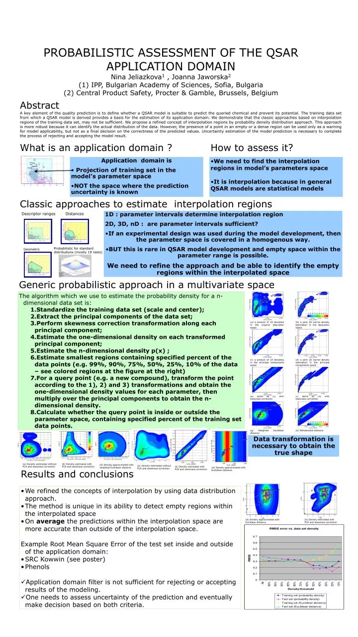
PROBABILISTIC ASSESSMENT OF THE QSAR APPLICATION DOMAINNina Jeliazkova1 , Joanna Jaworska2(1) IPP, Bulgarian Academy of Sciences, Sofia, Bulgaria (2) Central Product Safety, Procter & Gamble, Brussels, Belgium Descriptor ranges Distances (a) a product of 1D densities in the original descriptor space (b) a joint 2D kernel density estimation in the descriptor space (c) a product of 1D densities in the principal components space (d) a joint 2D kernel density estimation in the principal components space (e) same as (c) with skewness correction (f) same as (d) with skewness correction (g) Weighted Euclidean distance (e) Mahalanobis distance Abstract A key element of the quality prediction is to define whether a QSAR model is suitable to predict the queried chemical and prevent its potential. The training data set from which a QSAR model is derived provides a basis for the estimation of its application domain. We demonstrate that the classic approaches based on interpolation regions of the training data set, may not be sufficient. We propose a refined concept of interpolation regions by probability density distribution approach. This approach is more robust because it can identify the actual distribution of the data. However, the presence of a point in an empty or a dense region can be used only as a warning for model applicability, but not as a final decision on the correctness of the predicted values. Uncertainty estimation of the model prediction is necessary to complete the process of rejecting and accepting the model result. What is an application domain ? How to assess it? • Application domain is • Projection of training set in the model’s parameter space • NOT the space where the prediction uncertainty is known • We need to find the interpolation regions in model’s parameters space • It is interpolation because in general QSAR models are statistical models Classic approaches to estimate interpolation regions • 1D : parameter intervals determine interpolation region • 2D, 3D, nD : are parameter intervals sufficient? • If an experimental design was used during the model development, then the parameter space is covered in a homogenous way. • BUT this is rare in QSAR model development and empty space within the parameter range is possible. • We need to refine the approach and be able to identify the empty regions within the interpolated space Probabilistic for standard distributions (mostly 1D tests) Geometric Generic probabilistic approach in a multivariate space • The algorithm which we use to estimate the probability density for a n-dimensional data set is: • Standardize the training data set (scale and center); • Extract the principal components of the data set; • Perform skewness correction transformation along each principal component; • Estimate the one-dimensional density on each transformed principal component; • Estimate the n-dimensional density p(x) ; • Estimate smallest regions containing specified percent of the data points (e.g. 99%, 90%, 75%, 50%, 25%, 10% of the data – see colored regions at the figure at the right) • For a query point (e.g. a new compound), transform the point according to the 1), 2) and 3) transformations and obtain the one-dimensional density values for each parameter, then multiply over the principal components to obtain the n-dimensional density. • Calculate whether the query point is inside or outside the parameter space, containing specified percent of the training set data points. Data transformation is necessary to obtain the true shape (a) Density estimated without PCA and skewness correction (b) Density estimated with PCA and skewness correction (d) Density approximated with weighted Euclidean distance (a) Density estimated without PCA and skewness correction (b) Density estimated with PCA and skewness correction (d) Density approximated with Euclidean distance Results and conclusions • We refined the concepts of interpolation by using data distribution approach. • The method is unique in its ability to detect empty regions within the interpolated space • On average the predictions within the interpolation space are more accurate than outside of the interpolation space. • Example Root Mean Square Error of the test set inside and outside of the application domain: • SRC Kowwin (see poster) • Phenols • Application domain filter is not sufficient for rejecting or accepting results of the modeling. • One needs to assess uncertainty of the prediction and eventually make decision based on both criteria. (d) Density approximated with Euclidean distance (b) Density estimated with PCA and skewness correction


