Download

1 / 31
310 likes | 600 Views
Microfoundations of Financial Economics 2004-2005 2 Choices under uncertainty - Equilibrium. Professor André Farber Solvay Business School Université Libre de Bruxelles. Preferences under uncertainty. Standard approach based on axioms of cardinal utility – von Neuman Morgenstern (VNM).

E N D
Microfoundations of Financial Economics2004-20052 Choices under uncertainty - Equilibrium Professor André Farber Solvay Business School Université Libre de Bruxelles
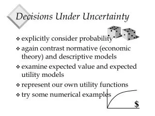
Preferences under uncertainty • Standard approach based on axioms of cardinal utility – • von Neuman Morgenstern (VNM). • Suppose Y is a random variable: {Y(s), π(s)} • u() is a cardinal utility function • u’(.) > 0 • u” attitude toward risk • risk lover u” >0 • risk neutral u” = 0 • risk averter u” <0 PhD 02
Example u(c)=ln(c) 40 1/2 c =10 1/2 PhD 02
Measuring risk aversion: ARA • Suppose Y = W + x E(x)=0 • What is the risk premium p such that: E[u(W+x)] = u(W – p) • Using Taylor expansion: Absolute risk aversion: PhD 02
Measuring risk aversion: RRA • Suppose now that the uncertainty is proportional to wealth: x = r W • Y = W(1+r) • As: Relative risk aversion: PhD 02
Quadratic utility function increasing increasing PhD 02
Exponential utility constant increasing PhD 02
Log utility decreasing constant PhD 02
Power utility decreasing constant PhD 02
What value for RRA? For an updated version see:Bliss and Panigirtzoglou, “Options-Implied Risk Aversion Estimates”, Journal of Finance, 59, 1 (Feb.2004) PhD 02
Demand for securities • Let’s first ignore c0 • Initial wealth: W • 2 security: riskless bond (gross return Rf) and risky asset (gross return R) • Let a be the amount invested in the risky asset Note: f’(a) = E[u’(c)(R – Rf)] and f”(a)<0 ???????? PhD 02
Optimum • a* > 0 f’(0)>0 u’(W)E(R - Rf) > 0 E(R) > Rf • FOC: PhD 02
Quadratic utility PhD 02
Exponential utility + normally distributed returns If z is normal: PhD 02
Log utility Suppose R can take two values: Ruwith proba πRdwith proba (1-π)Ru >Rf>Rd FOC: PhD 02
Power utility Suppose R can take two values: Ruwith proba πRdwith proba (1-π)Ru >Rf>Rd FOC: PhD 02
How does a change when W vary? • Decreasing absolute risk aversion implies da/dW>0 • Decreasing relative risk aversion implies that the fraction invested in the risky asset increases with wealth PhD 02
Two-period models of consumption decisions under uncertainty • Early models: Leland 1968, Sandmo • 1 risky asset • General representation of consumer’s preferences • U(c0,c1) = E[u(c0,c1)] • Budget constraint c0 + zp = W FOC: PhD 02
Utility: time-separable Von Neuman –Morgenstern function FOC: Remember p = E(mx) PhD 02
Numerical example (DD Chap 8) Endowment (Illustration using Excel file) PhD 02
Using power utility Suppose consumption growth is lognormal Define PhD 02
Understanding interest rates • Interest rates are high when: • People are impatient - δ high • In good times - E(Δln(c)) high - γ controls intertemporal substitution) • In safe times - σ²(Δln(c)) low -γ controls intertemporal substitution PhD 02
CCAPM Start from: Power utility: Assets pay a higher expected return if: covary negatively with m covary positively with consumption growth PhD 02
Looking at the data • Annual data US 1948-2002 (Source: Cochrane) percent E(R – Rf) σ(R) E(Δc) σ(Δc) corr(Δc,R) 7.21 18.0 1.31 1.93 0. 39 7.2 = γ×0.135 γ = 53!!! HUGE Equity premium puzzle (Mehra Prescott) PhD 02
Suppose γ = 53. What about Rf? Risk free rate Puzzle Either δ negative (people prefer future) or real interest rate = 17% + δ PhD 02
Toward a Mean Variance Frontier Start from: For ρi,m = +1: For ρi,m = -1: PhD 02
Mean-Variance Frontier Slope = PhD 02
Equity puzzle again Pick a frontier portfolio Rmv E(m) ≈ 1 and σ(m) = γσ(Δc) US, last 80 years: Sharpe ratio ≈ 0.50 and σ(Δc) ≈ 1% σ(m) = 50% Is this realistic ? (remember E(m) ≈ 1) γ≈ 50 This is the equity premium puzzle stated differently PhD 02
Hansen-Jagannathan Bounds E(R) σ(m) SR 1/E(m) E(m) σ(R) PhD 02
Hansen-Jagannathan bounds: recent estimates Lustig, Hanno N. and Van Nieuwerburgh, Stijn, "Housing Collateral, Consumption Insurance and Risk Premia: An Empirical Perspective" (March 15, 2004). EFA 2004 Maastricht Meetings Paper No. 1403. http://ssrn.com/abstract=556101 - also Journal of Finance June 2005 PhD 02
Tomorrow • CAPM: traditional derivations PhD 02