Download
1 / 15
160 likes | 703 Views
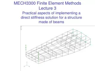
MECH3300 Finite element methods. Lecture 10 Issues in modelling Solving the equations. Use of symmetry.

E N D
MECH3300 Finite element methods Lecture 10 Issues in modelling Solving the equations
Use of symmetry • With increasing computer power, many analysts cannot be bothered with symmetry. However, there are always problems that are too big, that can be reduced in size at least 4 fold, by exploiting symmetry. • Even if loading is unsymmetric, symmetry of geometry can be exploited by subdividing the loading into symmetric and antisymmetric components and superimposing two solutions, modelling 1/2 the structure, and changing restraints on the plane of symmetry.. F F/2 F/2 F/2 F/2 Symmetric case Antisymmetric case Plane of symmetry
Restraints for modelling symmetry • With symmetric deformation, nodes in a plane of symmetry remain there. • To make this happen, fix displacement normal to the plane and rotations about axes in-plane (if defined). • Conversely, permit in-plane displacements and rotation about the normal to the plane of symmetry. • Anti-symmetry is the opposite - no motion in the plane of symmetry.
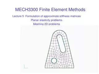
Meshing solid models • For machine components, it is possible to automatically mesh a CAD solid model. Standard formats are needed to import geometry into FE packages (eg IGES - International Graphic Exchange Standard). • Geometry needs to be checked, for duplicate edges, very short edges that would produce too fine a mesh locally, and for details that should be omitted, as it is not practical to mesh them. Geometry must be checked for free edges, or faces, to ensure it is connected properly. • A surface mesh is often created first with plates, and this used to guide generation of a solid mesh. • A mesh created by automatic or other meshing must be checked for duplicated nodes or elements, and to ensure all elements are connected correctly.
Example of auto-meshing inappropriate geometry (Strand7 tutorial problem) Nodes cluster to attempt to match 2 very short side-lengths present in the geometry - these “slivers” need removing. Some simplification of the real geometry is often needed to get an appropriate mesh.
Loading and restraining solid models A solid model subject to a point load will have very high stress at the load. This makes it impossible to see the stress elsewhere on a contour plot, and is unrealistic. Hence loads must be distributed realistically. This can take some thought - eg loading due to a pin in a hole. Distribution? Quadratic by Hertz theory. Restraints also need realistic distribution. For the pin in a hole case, polar coordinates at the centre of the hole are needed so as to fix radial displacements around the hole, but not tangential ones. Over what angle of arc?
Meshing arbitrary shapes • This is something commercial packages still not not do well. • A surface described by a stereolithography *.stl file can often be imported, but this can be a very fine triangulation. It may be possible to “unrefine” this to get a more suitable mesh (the command exists in NASTRAN for Windows for instance), but this may still take much to long to do to be practical.
Equation solvers • The large set of equations in a linear elastic finite element model is solved either by Gauss elimination or by an iterative algorithm (eg the pre-conditioned conjugate gradient method). • The iterative solvers tend to become more efficient on very large problems. (eg 100000 nodes). They use sparse matrix storage, that is they store only non-zero terms along with their row and column addresses. • There are different ways of organizing how Gauss elimination is done. • It is always 2 stages - triangular decomposition [K] = [L][U], followed by back-substitution F = [L]z, z = [U]u. • (a) the equations can be written in an order that minimizes the bandwidth of [K], so that only terms within the bandwidth are stored on disk or processed by the solver. • (b) the “wavefront” solver, implemented in ANSYS can be used.
The wavefront solver • In this approach to solving the equations, the elements are numbered so that elements connected together have similar numbers. Only those elements connected to a node having its equations processed must be assembled at any one time. • The effect of solving equations one node at a time is that the mesh is divided into 3 regions - nodes yet to be processed, nodes being processed, and nodes having been processed. • The boundaries between these regions sweep across the mesh, hence the “wavefront” name. • This approach may be more efficient than a bandwidth -minimizing solver.
Explicit Solvers One approach to highly nonlinear problems is to integrate in time using Newton’s law ie FEXT+ FINT = Ma FEXT = external forces (applied loads) at some time. FINT= internal forces (due to elastic or plastic deformation etc.) M = mass matrix a = accelerations - solve for these. If M is diagonal, then these are found “explicitly” from the forces. The new accelerations give new velocities and displacements (central difference method). These are used to find new internal forces, and to again to find new accelerations, and so on. Timestep size must be very small (eg microseconds).
Substructures or superelements • Traditionally, very large models of ships, cars bodies etc. were solved by a divide and conquer approach of separating the mesh into different regions called either substructures or superelements. • The equations for each region are “statically condensed” to give many fewer equations just relating forces/displacements on the interfaces between regions. • These are solved, and the interface displacements provide boundary conditions to solve the equations for each substructure separately. • A typical substructure would be the wing of an aircraft - the rear fuselage may be another, and the tail a third etc. • These methods are still used where a model of part of a system is prepared by a sub-contractor - eg a payload for the space shuttle.
Eigenvalue problems • Finding critical loads for buckling, or finding natural frequencies for vibration leads to matrix eigenvalue problems. • For undamped natural frequencies [K]u =l[M]umust be solved,where [M] is a mass matrix and the eigenvalue l is the angular natural frequency squared w2- more next semester in dynamics. • For buckling [K]u =l[Kg]u where [Kg] is a geometric stiffness matrix describing the change in stiffness due to finite deformation, worked out for the loading used previously in a linear static analysis. • The eigenvalue l this time is a factor on the loading that will scale it up to that causing buckling. • This approach is as accurate as hand calculation of a critical load, but not a true finite deformation analysis that keeps updating coordinates of nodes - it is just a perturbation of a linear analysis.
Solving eigenvalue problems • We usually only want to know the lowest natural frequencies of a vibrating structure, as they are most easily excited. • Similarly, only the lowest buckling eigenvalue is meaningful, as it takes less work to make the structure collapse at this load, than at the others predicted, which could only occur if buckling were prevented at the lowest critical load. • Hence the most appropriate solvers are algorithms that iteratively refine estimates of u to find the lowest modes of deformation. These can however, potentially miss a solution in an ill-conditioned problem. An algorithm which counts how many eigenvalues exist in a particular range of values can be used to check if solutions are missing (a Sturm sequence check). • The user can typically select how many modes of deformation to estimate. The results are usually animated to see the motion more clearly.
Solving non-linear problems • Non-linear problems take much more computation to solve than static problems, as the solvers work by successive linearization, that is, the solution keeps going off on a tangent and is then corrected. • A static finite deformation analysis, for instance, is typically done by incrementing the loading a number of times. Within each load increment, “equilibrium iterations” are performed to correct the error between the external loads and the predictions of internal loads, found from the latest linearized solution. • The number of iterations, to predict a substantial change of shape can be many hundreds, and the equivalent of a linear static analysis is done every iteration. • A solution for the post-buckled state of a structure can be quite hard to obtain.
History of load-deflection in some element Equilibrium iterations • The progress of a non-linear solution can be pictured by the history of loading in a particular element versus its deflection. Load (eg tension in a particular bar) True load-deflection graph First load increment Deflection magnitude