Binary Search Trees

1. Binary Search Trees Comp 122, Spring 2004

2. Binary Trees 26 200 28 190 213 18 12 24 27 • Recursive definition • An empty tree is a binary tree • A node with two child subtrees is a binary tree • Only what you get from 1 by a finite number of applications of 2 is a binary tree. Is this a binary tree? 56 Comp 122, Spring 2004

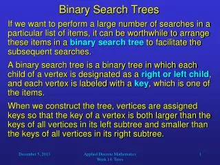
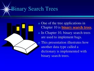
3. Binary Search Trees • View today as data structures that can support dynamic set operations. • Search, Minimum, Maximum, Predecessor, Successor, Insert, and Delete. • Can be used to build • Dictionaries. • Priority Queues. • Basic operations take time proportional to the height of the tree – O(h). Comp 122, Spring 2004

4. BST – Representation • Represented by a linked data structure of nodes. • root(T) points to the root of tree T. • Each node contains fields: • key • left – pointer to left child: root of left subtree. • right – pointer to right child : root of right subtree. • p – pointer to parent. p[root[T]] = NIL (optional). Comp 122, Spring 2004

5. Binary Search Tree Property Stored keys must satisfy the binary search tree property. y in left subtree of x, then key[y]  key[x]. y in right subtree of x, then key[y]  key[x]. 26 200 28 190 213 18 12 24 27 56 Comp 122, Spring 2004

6. Inorder Traversal 26 200 28 190 213 18 12 24 27 The binary-search-tree property allows the keys of a binary search tree to be printed, in (monotonically increasing) order, recursively. Inorder-Tree-Walk (x) 1. ifx NIL 2. then Inorder-Tree-Walk(left[p]) 3. print key[x] 4. Inorder-Tree-Walk(right[p]) 56 • How long does the walk take? • Can you prove its correctness? Comp 122, Spring 2004

7. Correctness of Inorder-Walk • Must prove that it prints all elements, in order, and that it terminates. • By induction on size of tree. Size=0: Easy. • Size >1: • Prints left subtree in order by induction. • Prints root, which comes after all elements in left subtree (still in order). • Prints right subtree in order (all elements come after root, so still in order). Comp 122, Spring 2004

8. Querying a Binary Search Tree • All dynamic-set search operations can be supported in O(h) time. • h = (lg n) for a balanced binary tree (and for an average tree built by adding nodes in random order.) • h =(n) for an unbalanced tree that resembles a linear chain of n nodes in the worst case. Comp 122, Spring 2004

9. Tree Search 26 200 28 190 213 18 56 12 24 27 Tree-Search(x, k) 1. ifx =NIL or k = key[x] 2. then return x 3. ifk <key[x] 4. then return Tree-Search(left[x], k) 5. else return Tree-Search(right[x], k) Running time: O(h) Aside: tail-recursion Comp 122, Spring 2004

10. Iterative Tree Search 26 200 28 190 213 18 56 12 24 27 Iterative-Tree-Search(x, k) 1. whilex  NILandk  key[x] 2. doifk <key[x] 3. thenx left[x] 4. elsex right[x] 5. returnx The iterative tree search is more efficient on most computers. The recursive tree search is more straightforward. Comp 122, Spring 2004

11. Finding Min & Max • The binary-search-tree property guarantees that: • The minimum is located at the left-most node. • The maximum is located at the right-most node. Tree-Minimum(x)Tree-Maximum(x) 1. whileleft[x] NIL 1. whileright[x] NIL 2. dox left[x] 2. dox right[x] 3. returnx 3. returnx Q: How long do they take? Comp 122, Spring 2004

12. Predecessor and Successor • Successor of node x is the node y such that key[y] is the smallest key greater than key[x]. • The successor of the largest key is NIL. • Search consists of two cases. • If node x has a non-empty right subtree, then x’s successor is the minimum in the right subtree of x. • If node x has an empty right subtree, then: • As long as we move to the left up the tree (move up through right children), we are visiting smaller keys. • x’s successor y is the node that x is the predecessor of (x is the maximum in y’s left subtree). • In other words, x’s successor y, is the lowest ancestor of x whose left child is also an ancestor of x. Comp 122, Spring 2004

13. Pseudo-code for Successor 26 200 28 190 213 18 56 12 24 27 Tree-Successor(x) • if right[x] NIL 2. then return Tree-Minimum(right[x]) 3. yp[x] 4. whiley  NIL and x = right[y] 5. dox y 6. yp[y] 7. returny Code for predecessor is symmetric. Running time:O(h) Comp 122, Spring 2004

14. BST Insertion – Pseudocode Tree-Insert(T, z) y NIL x  root[T] whilex  NIL doy  x ifkey[z] < key[x] thenx  left[x] elsex  right[x] p[z]  y if y = NIL thenroot[t]  z elseifkey[z] < key[y] then left[y]  z elseright[y]  z Change the dynamic set represented by a BST. Ensure the binary-search-tree property holds after change. Insertion is easier than deletion. 26 200 28 190 213 18 56 12 24 27 Comp 122, Spring 2004

15. Analysis of Insertion Initialization:O(1) While loop in lines 3-7 searches for place to insert z, maintaining parent y.This takes O(h) time. Lines 8-13 insert the value: O(1)  TOTAL: O(h) time to insert a node. Tree-Insert(T, z) • y NIL • x  root[T] • whilex  NIL • doy  x • ifkey[z] < key[x] • thenx  left[x] • elsex  right[x] • p[z]  y • if y = NIL • thenroot[t]  z • elseifkey[z] < key[y] • then left[y]  z • elseright[y]  z Comp 122, Spring 2004

16. Exercise: Sorting Using BSTs Sort (A) for i 1 to n do tree-insert(A[i]) inorder-tree-walk(root) • What are the worst case and best case running times? • In practice, how would this compare to other sorting algorithms? Comp 122, Spring 2004

17. Tree-Delete (T, x) if x has no children  case 0 then remove x if x has one child  case 1 then make p[x] point to child if x has two children (subtrees)  case 2 then swap x with its successor perform case 0 or case 1 to delete it  TOTAL: O(h) time to delete a node Comp 122, Spring 2004

18. Deletion – Pseudocode Tree-Delete(T, z) /* Determine which node to splice out: either z or z’s successor. */ • if left[z] = NIL or right[z] = NIL • theny  z • elsey  Tree-Successor[z] /* Set x to a non-NIL child of x, or to NIL if y has no children. */ • ifleft[y]  NIL • then x  left[y] • elsex  right[y] /* y is removed from the tree by manipulating pointers of p[y] and x */ • if x  NIL • thenp[x]  p[y] /* Continued on next slide */ Comp 122, Spring 2004

19. Deletion – Pseudocode Tree-Delete(T, z) (Contd. from previous slide) • if p[y] = NIL • thenroot[T]  x • else if y  left[p[i]] • then left[p[y]]  x • else right[p[y]]  x /* If z’s successor was spliced out, copy its data into z */ • ify  z • then key[z]  key[y] • copy y’s satellite data into z. • returny Comp 122, Spring 2004

20. Correctness of Tree-Delete • How do we know case 2 should go to case 0 or case 1 instead of back to case 2? • Because when x has 2 children, its successor is the minimum in its right subtree, and that successor has no left child (hence 0 or 1 child). • Equivalently, we could swap with predecessor instead of successor. It might be good to alternate to avoid creating lopsided tree. Comp 122, Spring 2004

21. Binary Search Trees • View today as data structures that can support dynamic set operations. • Search, Minimum, Maximum, Predecessor, Successor, Insert, and Delete. • Can be used to build • Dictionaries. • Priority Queues. • Basic operations take time proportional to the height of the tree – O(h). Comp 122, Spring 2004

22. Red-black trees: Overview • Red-black trees are a variation of binary search trees to ensure that the tree is balanced. • Height is O(lg n), where n is the number of nodes. • Operations take O(lg n) time in the worst case. Comp 122, Spring 2004

23. Red-black Tree • Binary search tree + 1 bit per node: the attribute color, which is either red or black. • All other attributes of BSTs are inherited: • key, left, right, and p. • All empty trees (leaves) are colored black. • We use a single sentinel, nil, for all the leaves of red-black tree T, with color[nil] = black. • The root’s parent is also nil[T ]. Comp 122, Spring 2004

24. Red-black Tree – Example nil[T] 26 17 41 30 47 38 50 Comp 122, Spring 2004

25. Red-black Properties • Every node is either red or black. • The root is black. • Every leaf (nil) is black. • If a node is red, then both its children are black. • For each node, all paths from the node to descendant leaves contain the same number of black nodes. Comp 122, Spring 2004

26. Height of a Red-black Tree • Height of a node: • Number of edges in a longest path to a leaf. • Black-height of a node x, bh(x): • bh(x)is the number of black nodes (including nil[T ]) on the path from x to leaf, not counting x. • Black-height of a red-black tree is the black-height of its root. • By Property 5, black height is well defined. Comp 122, Spring 2004

27. Height of a Red-black Tree Example: Height of a node: Number of edges in a longest path to a leaf. Black-height of a node bh(x)is the number of black nodes on path from x to leaf, not counting x. h=4 bh=2 26 h=3 bh=2 h=1 bh=1 17 41 h=2 bh=1 h=2 bh=1 30 47 h=1 bh=1 38 h=1 bh=1 50 nil[T] Comp 122, Spring 2004

28. Hysteresis : or the value of lazyness • Hysteresis, n. [fr. Gr. to be behind, to lag.] a retardation of an effect when the forces acting upon a body are changed (as if from viscosity or internal friction); especially: a lagging in the values of resulting magnetization in a magnetic material (as iron) due to a changing magnetizing force Comp 122, Spring 2004