Download
1 / 50
520 likes | 776 Views
Projective Visual Hulls. Svetlana Lazebnik Beckman Institute University of Illinois. Joint work with . Edmond Boyer INRIA Rh ô ne-Alpes. Jean Ponce Beckman Institute. What Is a Visual Hull?. The visual hull of an object with respect to a set of input views is…

E N D
Projective Visual Hulls Svetlana Lazebnik Beckman Institute University of Illinois Joint work with Edmond Boyer INRIA Rhône-Alpes Jean Ponce Beckman Institute
What Is a Visual Hull? • The visual hullof an object with respect to a set of input views is… • The maximal shape that yields the same silhouettes as the original object in all the input views. • The intersection of the solid visual cones formed by back-projecting the silhouettes in all the input views.
Visual Hull: A 2D Example O1 O2 O3
Previous Work • Theory • Laurentini ’94, Petitjean ’98, Laurentini ’99 • Solid cone intersection: • Baumgart ’74 (polyhedra), Szeliski ’93 (octrees) • Image-based visual hulls • Matusik et al. ’00, Matusik et al. ’01 • Advanced modeling • Sullivan & Ponce ’98, Cross & Zisserman ’00, Matusik et al. ’02 • Applications • Leibe et al. ’00, Lok ’01, Shlyakhter et al. ’01
This Talk • S. Lazebnik, E. Boyer, and J. Ponce. ‘‘On Computing Exact Visual Hulls of Solids Bounded by Smooth Surfaces,’’ CVPR 2001. • Key contributions: • Computing the visual hull based on weakly calibrated cameras • Exact boundary representations • The rim mesh • The visual hull mesh • Mathematical techniques • Oriented Projective Geometry [Stolfi ’91] • Projective Differential Geometry
Frontier Point How Do Visual Cones Intersect?
Intersection Points Frontier Points How Do Visual Cones Intersect?
How Do Visual Cones Intersect? Cone Strips
Vertices: frontier points + intersection points Edges: intersection curve segments Faces: visual cone patches Visual Hull Mesh Visual Hull As Topological Polyhedron
Vertices: frontier points Edges: rim segments Faces: regions on the surface of the object Rim Mesh The Arrangement of Rims on the Surface of the Object
Image-Based Computation Weak calibration is sufficient The visual hull is an (oriented) projective construction
Rim Mesh Example 104 frontier points
Use transfer for reprojection Tracing Intersection Curves
The Egg (synthetic, 6 views) 24 frontier points, 44 triple points
Summary • Exact visual hulls: geometric and topological representations • The rim mesh • The visual hull mesh • Oriented projective framework • Weak calibration is enough for an image-based algorithm to compute the visual hull
Oriented Projective Geometry • Motivation: real cameras see only what is in front of them • Conventional projective space: Pn = (Rn+1 – {0}) / ~ x ~ y iff x = ay, a 0. • Oriented projective space: Tn = (Rn+1 – {0}) / ~ x ~ y iff x = ay, a> 0. • Two-sided model of the image plane Back range Front range The line at infinity
Example: Orienting Epipolar Lines X xj xi ej ei Oi Oj A simple case
Example: Orienting Epipolar Lines X Wrong! xj xi ej ei Oi Oj We’re in trouble
Example: Orienting Epipolar Lines X Flip orientation of the epipole xj xi ej ei Oi Oj Correct solution
Rediscovering ProjectiveDifferential Geometry • Motivation: projective reconstruction of smooth curves and surfaces • A surface in P3 (in homogeneous coordinates): x(u,v) = (x1(u,v), x2(u,v), x3(u,v), x4(u,v))T • A projective differential property is a property that remains invariant under the following transformations: • Rescaling of the homogeneous coordinatesa(u,v) x(u,v) • Reparametrization x(u(s,t), v(s,t)) • Projective transformation Mx(u,v)
Projective Differential Property: Local Shape From [Pae & Ponce, ‘99] Elliptic K > 0 Hyperbolic K < 0 Parabolic K = 0 K = LN – M2 L = |x, xu, xv, xuu|, M = |x, xu, xv, xuv|, N = |x, xu, xv, xvv|.
Projective Differential Property: Local Shape Elliptic: No asymptotic tangents Parabolic: One asymptotic tangent Hyperbolic: Two asymptotic tangents
Oriented Projective Differential Geometry (Curves in 2) • A curve in T2 (in homogeneous coordinates): x(t) = (x1(t), x2(t), x3(t))T • An oriented projective differential property is a property that remains invariant under the following transformations: • Rescaling of the homogeneous coordinates by a positive function a(t)x(t), a(t) > 0 • Orientation-preserving change of parameterx(t(s)), dt/ds > 0 • Orientation-preserving projective transformationMx(t), det M > 0
An Oriented Projective Differential Property Inflection k= 0 Concave Point k < 0 Convex Point k > 0 k = |x, x, x|
Koenderink’s Theorem: sgn K = sgn k Parabolic Hyperbolic Elliptic Inflection Concave Convex
Application: Rim Ordering X Ri Rj xi xj li lj Oi Oj
Application: Rim Ordering X Ri Rj xi xj ti tj Oi Oj
Rim Ordering Rj Ri X X Rj Ri k (ti li) > 0 k (ti li) < 0
Rim Ordering and Local Shape Rj Ri Ri Rj Oi Oi Oj Oj Elliptic Hyperbolic
References • Oriented Projective Geometry • Framework: Stolfi ’91 • Applications to computer vision: Laveau & Faugeras ’96, Hartley ’98, Werner & Pajdla ’00, Werner & Pajdla ’01 • Projective Differential Geometry • Textbooks: Lane ’32, Bol ’50 (3 volumes, in German)