Download
1 / 51
540 likes | 1.04k Views
Overview of Graph Theory. Ad Hoc Networking Instructor: Carlos Pomalaza-Ráez Fall 2003 University of Oulu, Finland. Some applications of Graph Theory. Models for communications and electrical networks Models for computer architectures

E N D
Overview of Graph Theory Ad Hoc Networking Instructor: Carlos Pomalaza-RáezFall 2003University of Oulu, Finland
Some applications of Graph Theory • Models for communications and electrical networks • Models for computer architectures • Network optimization models for operations analysis, including scheduling and job assignment • Analysis of Finite State Machines • Parsing and code optimization in compilers
Application to Ad Hoc Networking • Networks can be represented by graphs • The mobile nodes are vertices • The communication links are edges Vertices Edges • Routing protocols often use shortest path algorithms • This lecture is background material to the routing algorithms
Elementary Concepts • A graph G(V,E) is two sets of object • Vertices (or nodes) , set V • Edges, set E • A graph is represented with dots or circles (vertices) joined by lines (edges) • The magnitude of graph G is characterized by number of vertices |V| (called the order of G) and number of edges |E| (size of G) • The running time of algorithms are measured in terms of the order and size
Directed Graph An edge e E of a directed graph is represented as an ordered pair (u,v), where u, v V. Here u is the initial vertex and v is the terminal vertex. Also assume here that u ≠ v 2 3 1 4 V = { 1, 2, 3, 4}, | V | = 4 E = {(1,2), (2,3), (2,4), (4,1), (4,2)}, | E|=5
Undirected Graph An edge e E of an undirected graph is represented as an unordered pair (u,v)=(v,u), where u, v V. Also assume that u ≠ v 2 3 1 4 V = { 1, 2, 3, 4}, | V | = 4 E = {(1,2), (2,3), (2,4), (4,1)}, | E|=4
Degree of a Vertex Degree of a vertex in an undirected graph is the number of edges incident on it. In a directed graph, the out degreeof a vertex is the number of edges leaving it and the in degree is the number of edges entering it 2 2 3 3 1 1 4 4 The indegree of vertex 2 is 2 and the in degree of vertex 4 is 1 The degree of vertex 2 is 3
Weighted Graph A weighted graph is a graph for which each edge has an associated weight, usually given by a weight functionw: E R 2 2 2 0.5 4 1.2 6 3 3 1 1 0.2 9 8 2.1 4 4
Walks and Paths 3 V2 V3 1 2 3 V1 1 V6 4 4 V5 V4 1 A walk is an sequence of nodes (v1, v2,..., vL) such that{(v1, v2), (v1, v2),..., (v1, v2)} E, e.g. (V2, V3,V6, V5,V3) A simplepath is a walk with no repeated nodes, e.g. (V1, V4,V5, V2,V3) A cycle is an walk (v1, v2,..., vL) where v1=vL with no other nodes repeated and L>3, e.g. (V1, V2,V5, V4,V1) A graph is called cyclic if it contains a cycle; otherwise it is called acyclic
Complete Graphs A complete graph is an undirected/directed graph in which every pair of vertices is adjacent. If (u, v ) is an edge in a graph G, we say that vertex v is adjacent to vertex u. A A B B C C D 4 nodes and (4*3)/2 edges V nodes and V*(V-1)/2 edges 3 nodes and 3*2 edges V nodes and V*(V-1) edges
Connected Graphs An undirected graph is connected if you can get from any node to any other by following a sequence of edges OR any two nodes are connected by a path B C A E F D A B A directed graph is strongly connected if there is a directed path from any node to any other node C D • A graph is sparse if | E | | V | • A graph is dense if | E | | V |2
Bipartite Graph V1 A bipartite graphis an undirected graphG = (V,E) in which V can be partitioned into 2 sets V1 and V2 such that ( u,v) E implies eitheruV1 and vV2 OR vV1 and u V2. V2 u1 v1 u2 v2 u3 v3 u4 An example of bipartite graph application to telecommunication problems can be found in, C.A. Pomalaza-Ráez, “A Note on Efficient SS/TDMA Assignment Algorithms,” IEEE Transactions on Communications, September 1988, pp. 1078-1082. For another example of bipartite graph applications see the slides in the Addendum section
Trees • Let G = (V, E ) be an undirected graph. • The following statements are equivalent, • G is a tree • Any two vertices in G are connected by unique simple path • G is connected, but if any edge is removed from E, the resulting graph is disconnected • G is connected, and | E | = | V | -1 • G is acyclic, and | E | = | V | -1 • G is acyclic, but if any edge is added to E, the resulting graph contains a cycle A C B D E F
Spanning Tree A tree (T ) is said to span G = (V,E) if T = (V,E’) and E’ E V2 For the graph shown on the right two possible spanning trees are shown below V3 V6 V1 For a given graph there are usually several possible spanning trees V5 V4 V2 V3 V2 V3 V6 V1 V1 V6 V4 V4 V5 V5
Minimum Spanning Tree Given connected graph G with real-valued edge weights ce, a Minimum Spanning Tree (MST) is a spanning tree of G whose sum of edge weights is minimized 3 2 3 2 24 4 4 1 1 23 9 9 6 6 18 6 6 4 4 5 5 11 11 16 5 5 8 8 7 7 14 10 7 7 8 8 21 G = (V, E) T = (V, F) w(T) = 50 Cayley's Theorem (1889) There are nn-2 spanning trees of a complete graph Kn • n = |V|, m = |E| • Can't solve MST by brute force (because of nn-2)
Applications of MST MST is central combinatorial problem with diverse applications • Designing physical networks • telephone, electrical, hydraulic, TV cable, computer, road • Cluster analysis • delete long edges leaves connected components • finding clusters of quasars and Seyfert galaxies • analyzing fungal spore spatial patterns • Approximate solutions to NP-hard problems • metric TSP (Traveling Salesman Problem), Steiner tree • Indirect applications. • describing arrangements of nuclei in skin cells for cancer research • learning salient features for real-time face verification • modeling locality of particle interactions in turbulent fluid flow • reducing data storage in sequencing amino acids in a protein
MST Computation Prim’s Algorithm • Select an arbitrary node as the initial tree (T) • Augment T in an iterative fashion by adding the outgoing edge (u,v), (i.e., u T and v G-T ) with minimum cost (i.e., weight) • The algorithm stops after |V | - 1 iterations • Computational complexity = O (|V|2) Kruskal’s Algorithm • Select the edge e E of minimum weight → E’ = {e} • Continue to add the edge e E – E’ of minimum weight that when added to E’, does not form a cycle • Computational complexity = O (|E|xlog|E|)
Prim’s Algorithm (example) V2 3 V3 V1 V2 V3 Algorithm starts 1 2 3 V6 V2 3 V1 1 1 1 4 3 1 V1 4 V1 V5 V4 After the 2nd iteration After the 1st iteration V3 V3 V2 V2 3 V2 3 3 V3 1 1 1 2 3 1 1 1 V1 V1 V1 V6 1 1 V4 V5 V4 V5 V5 After the 5th iteration After the 3rd iteration After the 4th iteration
Kruskal’s Algorithm (example) V2 3 V3 V2 V3 V2 1 2 1 1 3 1 After the 1stiteration V6 V1 1 V1 V1 4 1 V4 4 V2 V3 V5 1 V4 V5 1 V1 1 After the 2nditeration After the 3rd iteration V5 V2 V2 V3 3 V3 1 1 2 2 1 1 V1 V1 V6 V6 1 1 V5 V4 V5 V4 After the 4th iteration After the 5th iteration
Distributed Algorithms • Each node does not need complete knowledge of the topology • The MST is created in a distributed manner • Example of this type of algorithms is the one proposed by Gallager, Humblet, and Spira (“Distributed Algorithm for Minimum-Weight Spanning Trees,” ACM Transactions on Programming Languages and Systems, January 1983, pp. 66-67). • Starts with one or more fragments consisting of single nodes • Each fragment selects its minimum weight outgoing edge and using control messaging fragments coordinate to merge with a neighboring fragment over its minimum weight outgoing edge • The algorithm can produce a MST in O(|V |x|V |) time provided that the edge weights are unique • If these weights are not unique the algorithm still works by using the nodes IDs to break ties between edges with equal weight • The algorithm requires O(|V |xlog|V |) + |E |) message overhead
Distributed Algorithm- Example 1 V2 1 V2 V3 Zero level fragments V3 4 4 1 3 1 2 3 2 V6 5 5 V7 V7 V1 V6 5 V1 4 5 4 2 2 3 3 V5 V4 6 V5 V4 6 Nodes 3, 4, and 7 join fragment {1,2} 1 V2 1st level fragments {1,2} and {5,6} are formed 1 V2 V3 V3 4 1 3 4 2 1 3 2 5 5 V7 V7 V6 V1 5 V6 4 V1 5 4 2 3 2 3 V5 V5 V4 V4 6 6 1 V2 V3 Fragments {1,2,3,4,7} and {5,6} join to form 2nd level fragment that is the MST 4 1 3 2 5 V7 V6 V1 5 4 2 3 V4 V5 6
Shortest Path Spanning Tree A shortest path spanning tree (SPTS), T, is a spanning tree rooted at a particular node such that the |V |-1 minimum weight paths from that node to each of the other network nodes is contained in T 2 2 2 2 6 2 2 6 3 3 1 5 3 1 5 1 2 2 2 4 4 4 Shortest Path Spanning Treerooted at vertex 1 Minimum Spanning Tree Graph Note that the SPST is not the same as the MST
Applications of Trees • Unicast routing (one to one) → SPST • Multicast routing (one to several) • Maximum probability of reliable one to all communications → maximum weight spanning tree • Load balancing → Degree constrained spanning tree
Shortest Path Algorithms • Assume non-negative edge weights • Given a weighted graph (G, W ) and a node s, a shortest path tree rooted at s is a tree T such that, for any other node v G, the path between s and v in T is a shortest path between the nodes • Examples of the algorithms that compute these shortest path trees are Dijkstra and Bellman-Ford algorithms as well as algorithms that find the shortest path between all pairs of nodes, e.g. Floyd-Marshall
Dijkstra Algorithm Procedure (assume s to be the root node) V’ = {s}; U =V-{s};E’ = ;Forv U doDv = w(s,v);Pv = s;EndForWhileU≠ do Find v Usuch that Dv is minimal;V’ = V’{v}; U = U – {v};E’ = E’ (Pv,v);Forx U doIfDv + w(v,x) < DxthenDx = Dv + w(v,x);Px = v;EndIf EndForEndWhile
Example - Dijkstra Assume V1 is s and Dv is the distance from node s to node v. Ifthere is no edge connecting two nodes x and y→ w(x,y) = ∞ 1 V3 V2 4 1 3 2 5 V6 V1 V7 4 4 2 3 V5 V4 6 D3=∞ 1 1 D3=2 D2=1 V3 D2=1 V3 V2 V2 4 4 1 3 1 3 2 2 5 5 V6 V6 V1 D7=3 V7 V1 D7=∞ V7 4 D6=∞ 4 4 D6=∞ 4 3 3 2 2 V5 V4 V5 V4 6 6 D5=∞ D4=3 D5=∞ D4=3 V’= {1} V’= {1,2}
Example - Dijkstra 1 1 V3 V3 D2=1 D2=1 D3=2 D3=2 V2 V2 4 4 1 1 3 3 2 2 5 5 V6 V6 V1 V1 D7=3 V7 D7=3 V7 4 4 D6=6 D6=6 4 4 3 3 2 2 V5 V5 V4 V4 6 D5=9 6 D4=3 D5=∞ D4=3 V’= {1,2,3} V’= {1,2,3,4} 1 1 V3 D2=1 V3 D2=1 D3=2 D3=2 V2 V2 4 4 1 3 1 3 2 2 5 5 V6 V6 V1 D7=3 V7 V1 D7=3 V7 4 D6=6 4 4 D6=6 4 3 3 2 2 V5 V4 V5 V4 6 6 D5=7 D4=3 D5=7 D4=3 V’= {1,2,3,4,7} V’= {1,2,3,4,7,6}
Example - Dijkstra 1 V3 D2=1 D3=2 V2 The algorithm terminates when all the nodes have been processed and their shortest distance to node 1 has been computed 4 1 3 2 5 V6 V1 D7=3 V7 4 D6=6 4 3 2 V5 V4 6 D5=7 D4=3 V’= {1,2,3,4,7,6,5} 1 V3 V2 4 1 3 2 Note that the tree computed is not a minimum weight spanning tree. A MST for the given graph is → 5 V6 V1 V7 4 4 3 2 V5 V4 6
Bellman-Ford Algorithm Find the shortest walk from a source node s to an arbitrary destination node v subject to the constraints that the walk consist of at most h hops and goes through node v only once ProcedureDv-1= ∞ v V;Ds0= 0 and Dv0= ∞ v ≠ s, v V;h = 0;Until (Dvh= Dvh-1v V)or(h = |V |)doh = h + 1;Forv VdoDvh+1 = min{Duh + w(u,v)}u V;EndForEndUntil
Bellman-Ford Algorithm (Example) Until (Dvh= Dvh-1v V)or(h = |V |)doh = h + 1;Forv VdoDvh+1 = min{Duh + w(u,v)}u V;EndForEndUntil 1 V3 V2 4 1 3 2 5 V6 V1 V7 4 4 2 3 V5 V4 6 1 V3 V2 4 1 3 2 5 V6 V1 V7 4 4 2 3 V5 V4 6
Floyd-Warshall Algorithm Find the shortest path between all ordered pairs of nodes (s,v), {s,v} v V. Each iteration yields the path with the shortest weight between all pair of nodes under the constraint that only nodes {1,2,…n}, n |V |,can be usedas intermediary nodes on the computed paths. ProcedureD= W;(W isthe matrix representation of the edge weights)For u = 1to |V |doFor s = 1to |V |doFor v = 1to |V |doDs,v = min{Ds,v, Ds,u+ Wu,v}EndForEndForEndFor Note that this algorithm completes in O(|V |3) time
Floyd-Warshall Algorithm (Example) D= WFor u = 1to |V |doFor s = 1to |V |doFor v = 1to |V |doDs,v = min{Ds,v, Ds,u+ Wu,v}EndForEndForEndFor V2 2 2 2 8 6 V1 V3 4 1 1 4 3 3 1 V4 V5 5 V1 V2 V3 V4 V5 V1 V2 V3 V4 V5
Distributed Asynchronous Shortest Path Algorithms • Each node computes the path with the shortest weight to every network node • There is no centralized computation • As for the distributed MST algorithm described in [Gallager, Humblet, and Spiral], control messaging is required to distributed computation • Asynchronous means here that there is no requirement of inter-node synchronization for the computation performed at each node of for the exchange of messages between nodes
Distributed Dijkstra Algorithm • There is no need to change the algorithm • Each node floods periodically a control message throughout the network containing link state information → transmission overhead is O(|V |x|E|) • Entire topology knowledge must be maintained at each node • Flooding of the link state information allows for timely dissemination of the topology as perceived by each node. Each node has typically accurate information to be able to compute the shortest paths
Distributed Bellman-Ford Algorithm • Assume G contains only cycles of non-negative weight • If (u,v) E then so is (v,u) • The update equation is N(s) = Neighbors of s → • Each node only needs to know the weights of the edges that are incident to it, the identity of all the network nodes and estimates (received from its neighbors) of the distances to all network nodes
Distributed Bellman-Ford Algorithm • Each node s transmits to its neighbors its current distance vector Ds,V • Likewise each neighbor node u N(s) transmits to s its distance vector Du,V • Node s updates Ds,v, v V – {s} in accordance with:If any update changes a distance value then s sends the current version of Ds,vto its neighbors • Node s updates Ds,v every time that it receives a distance vector information from any of its neighbors • A periodic timer prompts node s to recomputeDs,V or to transmit a copy of Ds,V to each of its neighbors
Distributed Bellman-Ford AlgorithmExample 1 C B 7 A 8 2 1 D E 2 1 C B 7 A 8 2 1 D E 2 E receives D’s routes and updates its Ds,V
Distributed Bellman-Ford AlgorithmExample A receives B’s routes and updates its Ds,V 1 C B 7 A 8 2 1 D E 2 A receives E’s routes and updates its Ds,V 1 C B 7 A 8 2 1 D E 2
Distributed Bellman-Ford AlgorithmExample 1 C B 7 A 8 2 1 D E 2 1 C B 7 A 8 2 1 D E 2
Distance Vector Protocols • Each node maintains a routing table with entries{Destination, Next Hop, Distance (cost)} • Nodes exchange routing table information with neighbors • Whenever table changes • Periodically • Upon reception of a routing table from a neighbor a node updates its routing table if finds a “better” route • Entries in the routing table are deleted if they are too old, i.e. they are not “refreshed” within certain time interval by the reception of a routing table
Link Failure B Simple rerouting case E C A • F detects that link to G has failed • F sets a distance of ∞ to G and sends update to A • A sets a distance of ∞ to G since it uses F to reach G • A receives periodic update from C with 2-hop path to G (via D) • A sets distance to G to 3 and sends update to F • F decides it can reach G in 4 hops via A D F G
Link Failure B Routing loop case E • Link from A to E fails • A advertises distance of ∞ to E • B and C had advertised a distance of 2 to E (prior to the link failure) • Upon reception of A’s routing update B decides it can reach E in 3 hops; and advertises this to A • A decides it can read E in 4 hops; advertises this to C • C decides that it can reach E in 5 hops… C A D F G This behavior is called count-to-infinity
Count-to-Infinity Problem Example: routers working in stable state (A,1) (A,2) (A,3) (A,4) A B C D E (A,1) (A,2) (A,3) Routing updates with distances to A are shown
Count-to-Infinity Problem Example: link from A to B fails (A,2) (A,3) (A,4) A B C D E (A,3) (A,2) (A,3) updated information B can no longer reach A directly, but C advertises a distance of 2 to A and thus B now believes it can reach A via C and advertises it
Count-to-Infinity Problem After 2 exchanges of updates (A,4) (A,3) (A,4) A B C D E (A,3) (A,4) (A,3) After 3 exchanges of updates (A,4) (A,5) (A,4) A B C D E (A,5) (A,4) (A,5) After 4 exchanges of updates (A,6) (A,5) (A,6) A B C D E (A,5) (A,6) (A,5)
Count-to-Infinity Problem After 5 exchanges of updates (A,6) (A,7) (A,6) A B C D E (A,7) (A,6) (A,7) After 6 exchanges of updates (A,8) (A,7) (A,8) A B C D E (A,7) (A,8) (A,7) This continues until the distance to A reaches infinity
Split Horizon Algorithm • Used to avoid (not always) the count-to-infinity problem • If A routes to C via B, then A tells B that its distance to C is ∞ A B C (C,∞) B will not route to C via A if the link B to C fails • Works for two node loops • Does not work for loops with more than two nodes
Example Where Split Horizon Fails • When link C to D breaks, C marks D as unreachable and reports that to A and B. • Suppose A learns it first • A now thinks best path to D is through B • A reports D unreachable to B and a route of cost 3 to C • C thinks D is reachable through A at cost 4 and reports that to B. • B reports a cost 5 to A who reports new cost to C. • etc... B A C D