Download
1 / 55
640 likes | 1.11k Views
Ocean Modeling. Matt McKnight Boxuan Gu. Engineering the system. The Earth. Understanding that the Oceans are inextricably linked to the world ’ s climate is easy. Describing this relationship is more difficult, but starts from the basics. The Climate. Precipitation. Evaporation.

E N D
Ocean Modeling Matt McKnight Boxuan Gu
The Earth • Understanding that the Oceans are inextricably linked to the world’s climate is easy. • Describing this relationship is more difficult, but starts from the basics
The Climate Precipitation Evaporation
The Details • Without question we need a coupled atmospheric model • Taking into consideration other numerical models • Atmospheric Radiation • Solar Radiation • The sensible heat • Heat flux • Water density • Evaporation • Current • Wind stress • Temperature diffusion
Dynamic Models • Atmosphere • Larger spatial scale eddies • Much better observation • Globe-spanning • Ocean • Order of magnitude smaller eddies • Little data • Limited surface
Atmospheric Coupling • Interpolate between the atmosphere and ocean grids • Compute fluxes • Fresh water • Sensible heat • Latent heat • Sea Ice
The Ocean • We would like to have a very fine resolution <= 0.25 degrees because your average beach home doesn’t occupy much space on the map • Currents are more narrow at the poles and equator so we want even higher resolution
Ocean Floor • To be as accurate as possible, we would like to have details about the ocean floor. • The ocean floor is mostly unexplored and unmapped. Leaving many basic questions about the oceans unanswered
Ocean Floor • The knowledge of deep currents is currently very limited. • Modern systems use up 120 sound beams to produce maps up to 15 kilometers wide along a ship’s track • Satellite imaging is also used to resolve detail below the surface
Starting the Simulation • Due to little data from observations, especially sub-surface, we have initialization problems • Use only atmospheric data to start • Some models start with zero motion
Systematic Bias • Errors in the annual cycle • Climate drift depending on forecast lead time
Forecast model bias (Earth Simulator) • A comparison of the coupled model 12 month Nino3 forecasts [top panel] for February (blue), May (red), August (green), and November (brown) initial conditions average over all years, compared with climatology (purple). The bottom panel show the bias relative to this climatology. http://www.wmo.ch/web/wcp/clips2001/modules/21
Wavewatch III • A forecast from NOAA
Preface The first operational weather prediction occurred in May 1955 as a joint United States Air Force, Navy, and Weather Bureau project. In principle, numerical ocean modeling is similar to atmospheric modeling, but global operational oceanography has lagged far behind.
Atmospheric versus Oceanic Prediction Operational oceanography has lagged far behind atmospheric modeling because of two major complications. • First, oceanic space and time scales are much different than those of the atmosphere. • Second, unlike the meteorological radiosonde network that provides initial conditions from the surface to near the top of the atmosphere, there are few observations below the ocean surface at the synoptic time scale.
Cont. • Ocean eddies are typically 100 km in diameter, which makes them 20 to 30 times smaller than comparable atmospheric highs and lows. As a result, approximately four orders of magnitude more computer time and three orders of magnitude more computer memory are required.
Cont. • effective oceanic data assimilative techniques are limited to surface satellite observations, which were not available until the 1990s. One advantage ocean prediction enjoys is that forecast skill for many ocean features, including ocean eddies and the meandering of ocean currents and fronts, is longer than the 10 to 14 day limit for atmospheric pressure systems.
Cont. • as a nation protected from adversaries and linked to partners by the world's great oceans, it is fundamental that the US understand its surrounding marine environment. • Consequently, for the past decade, the NRL has been working on the problem of eddy-resolving global ocean modeling and prediction.
Cont. • Furthermore, it has developed the world's first global ocean nowcast and forecast system using the Department of Defense's High Performance Computing Modernization Program (HPCMP) computing resources. • It has been running in real time at the Naval Oceanographic Office (NAVO) since October 2000. Here, we describe the computational requirements of numerical ocean modeling and how the NRL system operates.
COMPUTATIONAL REQUIREMENTS • As far back as 1989, the President's Office of Science and Technology recognized global ocean modeling and prediction as a Grand Challenge problem, defined as requiring a computer system capable of sustaining at least one trillion floating-point adds or multiplies per second.
Cont. • NRL are solving the problem on today's systems capable of only a fraction of this performance by taking a multifaceted approach to cost minimization.
What they use ? • One facet is using the NRL Layered Ocean Model (NLOM),1 specifically designed for eddy-resolving global ocean prediction.
The advantages of NLOM • It is tens of times faster than other ocean models in computer time per model year for a given horizontal resolution and model domain. • NLOM's performance is due to a range of design decisions, the most important of which is the use of isopycnal (density-tracking) layers in vertical rather than fixed-depth cells.
Cont. • Density is the natural vertical coordinate system for the stratified ocean, and it lets seven NLOM layers replace the 50 or more fixed levels that would be needed at 1/16-degree (or 7 km mid-latitude) resolution. • NLOM's semi-implicit time scheme allows a longer time step by making it independent of all gravity waves.
Cont. • it requires solving a 2D Helmholtz's equation for each gravity mode at each time step. • NRL can solve internal modes with 5 to 10 red-black successive over-relaxation (SOR) sweeps, but efficient solution of the single external gravity mode requires direct solution using the Capacitance Matrix Technique(CMT).
Cont. • CMT involves solving a dense system of linear equations across all coastline points. This is a huge matrix for global regions (90,000 × 90,000 elements at 1/32-degree resolution). • However, it does not change with time, so we can invert it once at the start of the simulation, leaving a simple matrix-vector product to be performed at each time step.
Cont. • The NA824 benchmark consists of a typical NLOM simulation of three model days on a 1/32-degree five-layer Atlantic Subtropical Gyre region (grid size 2,048 × 1,344 × 5). • Like most heavily used benchmarks, this is for a problem smaller than those now typically run. The NA824 speedup from 28 to 56 processors is similar to the 112 to 224 speedup for the 1/64-degree Atlantic model, which is four times larger.
Figure 1. Performance of the NRL Layered Ocean Model NA824 benchmark on seven machines
Cont. • The sustained Mflops estimate is based on the number of floating-point operations reported by a hardware trace of a single-processor Origin 2000 run (without combined multiply-add operations) • that is, only useful flops (adds, multiplies, divides). A constant Mflops rate for all processor counts would indicate perfect scalability.
Cont. • Another facet of efficiency drive is the use of an inexpensive data assimilation scheme backed by a statistical technique for relating surface satellite data to subsurface fields. • The statistics are from an atmospherically forced 20-year interannual simulation of the same ocean model, an application that requires a model with high simulation skill.
Cont. • The NLOM system's focus on minimizing the computational cost is necessary if we are to provide near-global eddy-resolving capability on existing computers, but it comes at the price of relatively low vertical resolution and the exclusion of the Arctic (above 65 degrees North) and all coastal regions (shallower than 200 m).
Cont. • NRL is working on a second-generation global system without these limitations, but deployment is not scheduled until 2006 because of its much higher computational cost.
In October 2000, NRL achieved the major goal of Fiscal Year 1998-2000 HPC Challenge transitioning the world's first eddy-resolving nearly global (excluding the Arctic) ocean prediction system to NAVO for operational testing and evaluation. • NAVO made this NLOM-based system an operational Navy product in September 2001.
The system consists of the 1/16-degree seven-layer, thermodynamic, finite-depth version of the NLOM for the global ocean (72 degrees S to 65 degrees N) and includes a mixed layer and sea surface temperature (SST).
It was spun-up to real time using high-frequency wind and thermal forcing from the Fleet Numerical Meteorology and Oceanography Center's Navy Operational Global Atmospheric Prediction System (FNMOC's NOGAPS).
It assimilates SST plus real-time satellite altimeter data from three satellites using NAVO's Altimeter Data Fusion Center. • It runs in real time on 216 Cray T3E or IBM WinterHawk 2 processors, with daily updates and a 30-day forecast performed every Wednesday. It provides a real-time view of the ocean down to the 50 km to 200 km scale of ocean eddies and the meandering of ocean currents and fronts.
SSH NOWCAST COMPARISONS WITH FRONTAL ANALYSES • The NRL has developed evaluation software and has been monitoring the performance of the 1/16° global NLOM system to establish the baseline metrics for this first-generation operational system.
Cont. • One evaluation monitors the system's ability to nowcast the positions of major fronts and eddies on the global scale. • The War-fighting Support Center (WSC) at NAVO relies on satellite infrared (IR) SST data to locate fronts and eddies for the global ocean and release frontal analysis products to the fleet. The NLOM system lets the WSC analysis use daily nowcasts and animations of SSH to improve the quality of frontal analysis products.
Cont. • This is particularly significant because SSH is a better indicator of subsurface frontal location than SST. • Specifically, NLOM provides a daily map of the ocean mesoscale SSH field, which can help the WSC interpret cloud-filled IR images.
In addition, by using animations of the NLOM SSH field, analysts can better track front and eddy movements to help analyze the space and time continuity of the ocean mesoscale in areas where frontal analysis is required.
Cont. • The above figure is Sea-surface-height analysis (nowcast) in the Gulf Stream region from the real-time 1/16-degree global NRL Layered Ocean Model for (a) 4 June 2001 and (b) 11 June 2001. • Superimposed on each is an independent Gulf Stream north-wall frontal analysis determined from satellite IR imagery (white lines) by the Naval Oceanographic Office for the same days. • The color palette was chosen to emphasize the location of the Gulf Stream and associated eddies.
SSH(Sea surface height ) FORECASTS • NLOM's ability to forecast SSH and the positions of major fronts and eddies represents a new Naval product that can be used for future operational planning and to help users gauge the product's quality (by comparing forecasts with the analysis for that same day when it becomes available).
Cont. • The future positions of major ocean fronts will give the war-fighter some guidance on how changes in the ocean environment could affect future missions. • An accurate SSH forecast would let the Navy predict changes in locations of mesoscale features (fronts and eddies) that affect the 3D temperature and salinity field by using the predicted NLOM SSH and SST to derive synthetic profiles from the Modular Ocean Data Assimilation System.
The above figure is Sea surface height (cm) for the Kuroshio region from the 1/16-degree global NRL Layered Ocean Model running in forecast mode for a 30-day forecast.