Download
1 / 47
500 likes | 996 Views
Estimation of Porosity and Permeability from 4D-Seismic and Production Data Using Principal Component Analysis. Smart Fields Seminar Stanford University. July 31, 2008. Outline. The Norne Field The history matching problem Integrating production and seismic data The optimization problem

E N D
Estimation of Porosity and Permeability from 4D-Seismic and Production Data Using Principal Component Analysis Smart Fields Seminar Stanford University July 31, 2008
Outline • The Norne Field • The history matching problem • Integrating production and seismic data • The optimization problem • Principal Component Analysis • Results • Conclusions
Norne field • Discovered at 1991 • Size: 9 * 3 Km with 110 m oil and 75 m gas column • Seismic Survey: • Base: 1991 (Conventional) • 1th: July 2001 Q-Marine survey • 2th: August 2003 Q-Marine survey • 3th: August 2004 Q-Marine survey • 4th: August 2006 Q-Marine survey • 5th: July 2008 Q-Marine survey
Norne Simulation Model E • Model is redesigned based on 2004 geo model • 46 x 122 x 22, DX & DY~ 80-100 m • 46 development wells which only 22 are available • 15 producer • 8 injector D G C
Survey Difference 2003 - 2001 well CHT2
Semi Synthetic Model injector producer Permeability Porosity
Outline • The Norne Field • The history matching problem • Integrating production and seismic data • The optimization problem • Principal Component Analysis • Results • Conclusions
Inversion process Initial Guess (d) Response of the system M(θ*) Forward Modeling OPTIMIZATION min || M(θ)- M(θ*)|| Predicted parameters (K,Φ)
Outline • The Norne Field • The history matching problem • Integrating production and seismic data • The optimization problem • Principal Component Analysis • Results • Conclusions
Time-Lapse Seismic Data BASE MONITOR MONITOR-BASE
Am= f(X,∆V,∆ρ) (∆V,∆ρ)= f(T,Sf,P,C) X = Acquisition effects T = Temperature Sf = Fluid Saturation P = Pressure/Stress C = Compaction Assumptions: • No temperature variation • No Compaction Adding 4D seismic data Am Time(sec) • Variations in S and P affect 4D Am • Variations in K and affect S and P • Variations in K and affect 4D Am
Adding 4D seismic data Real 4D Seismic Processed 4D Seismic Real Production Data Sim. Production Data Sim Seismic Data Processing Match Petro Elastic model Reservoir Properties Flow Simulation ΔS, ΔP
Forward Models Used Production • Fluid Flow Simulation (Eclipse 100) Seismic • Petro Elastic Model • Gassmann’s equation (Saturation) • Hertz Mindlin Model (Pressure) • Forward seismic Modeling (Matrix propagation techniques)
Outline • The Norne Field • The history matching problem • Integrating production and seismic data • The optimization problem • Principal Component Analysis • Results • Conclusions
Objective Function Observed Data Production Seismic
Bound Constraints Geological bound Constraints
Four Optimization Strategies √ √ √ √ √ √ √ √ √ √ * production data is added after 15 iterations
All Strategies Reduce Cost Function P SZG ALT SZG+P
Production Matching WOPR WBHPI WBHPP WWPR
4D Seismic Matching Zero Offset Amplitude Mismatch AVO Gradients Mismatch 121% 140% 20% 20%
Estimated Porosity/Permeability Φ K Real Real Estimated Estimated
Estimated Porosity/Permeability porosity error permeability error
Outline • The Norne Field • The history matching problem • Integrating production and seismic data • The optimization problem • Principal Component Analysis • Results • Conclusions
Motivation for PCA • reduce CPU time • have a geologically acceptable estimate CPU-TIME=Number of forward Simulation x Number of Iterations expected
Principal Component Analysis • Orthogonal linear transformation • Other names: • Karhunen-Loeve Transform (KLT) • Proper Orthogonal Decomposition (POD) • Hotelling Transform • Involves eigenvalue decomposition / singular value decomposition of a covariance matrix • Application: • reduces dimension in multidimensional data sets • Introduces naturally geologic constraints
Principal Component Analysis • Interpretation as data compression orthonormal with and so that is maximized from D. Echeverria Ciaurri et al. 2008
Porosity Realizations • Matrix Approach: when size of the problem is huge • Turning Ban: has artifacts andconditioning to local data is difficult • Fractals: conditioning to local data is difficult • Annealing: recommended for permeability • Sequential Gaussian Simulation
Available Statistical Data • Log porosity of the wells • Permeability-porosity relation • Porosity distribution variogram
Sequential Gaussian Simulation • All conditional distribution is Gaussian and the mean and variance is given by kriging. Procedure • Transform data to normal scores • Establish grid network and coordinate system • Compute the variogram corresponding to available well data • Simulate realization by ordinary kriging which is conditioned to • variogram • local well data • … • Back transform all values
Realizations Porosity #1 Porosity #2 Porosity #3 Permeability #1 Permeability #2 Permeability #3
Effect of PCA (Porosity) Original 200 components Normalized variance 100 components 50 components Number of components
Effect of PCA (Permeability) Original 200 components Normalized variance 100 components 50 components Number of components
Optimization strategies using PCA PCA-STG1 PCA-STG2 i Optimization loop Optimization loop Iteration loop Iteration loop
Outline • The Norne Field • The history matching problem • Integrating production and seismic data • The optimization problem • Principal Component Analysis • Results • Conclusions
Estimated Porosity real porosity estimated porosity NOT-PCA estimated porosity PCA-STG1 estimated porosity PCA-STG2
Estimated Permeability estimated permeability NOT-PCA real permeability estimated permeability PCA-STG1 estimated permeability PCA-STG2
Outline • The Norne Field • The history matching problem • Integrating production and seismic data • The optimization problem • Principal Component Analysis • Results • Conclusions
Conclusions • Adding 4D seismic to production data yields a better history match • If geologic constraints are not considered, the matched solutions might not be geologically realistic • If numerical gradients are used in the history matching, the computational load can be prohibitive for practical applications
Conclusions • By Principal Component Analysis (PCA) we can speed up the gradient-based optimization considerably and at the same time take into account geologicconstraints • The good results obtained with this PCA-based technique in a semi synthetic case from the Norne field encourage to apply to the history matching of the complete field
Future Work • Apply PCA-based optimization to the complete field • Use distributed computing in gradient approximation • Test alternative optimization algorithms • Study efficient methods (adjoints) for gradient computation • Extension of PCA to Kernel PCA
Acknowledgements Stanford NTNU NFR • STATOIL for permission to use the reservoir model • Schlumberger-GeoQuest for the use of the Eclipse simulator. • Alexey Stovas (NTNU) for the seismic forward modeling • Jan Ivar Jensen (NTNU) For assistance
Estimation of Porosity and Permeability from 4D-Seismic and Production Data Using Principal Component Analysis Smart Fields Seminar Stanford University July 31, 2008