Download
1 / 35
370 likes | 839 Views
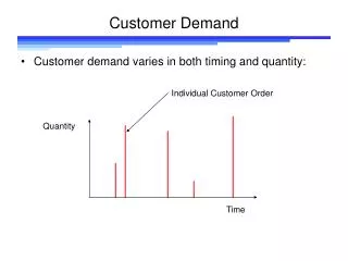
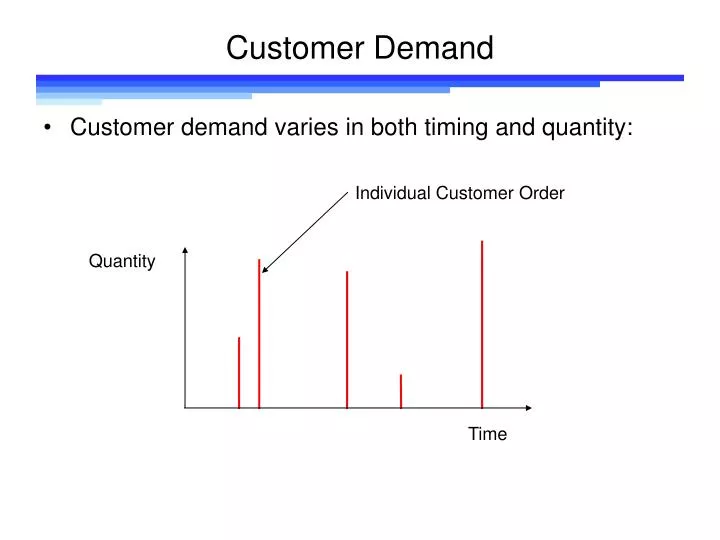
Customer Demand. Customer demand varies in both timing and quantity:. Individual Customer Order. Quantity. Time. Customer Demand.

E N D
Customer Demand • Customer demand varies in both timing and quantity: Individual Customer Order Quantity Time
Customer Demand • If demand for a product comes from many, independent customers, then we don’t need to be concerned about individual customer orders, but rather cumulative demand over a period of time.
Customer Demand Cumulative Demand for Period Individual Customer Demand Day 3 Day 4 Day 5 Day 6 Day 7 Day 8 Day 9 Day 1 Day 2 Demand
Customer Demand • In statistics, when there is reason to suspect the presence of a large number of small effects acting additively and independently, it is reasonable to assume that the observations will be normally distributed. • Therefore, if demand for a product comes from many, independent customers, we can assume that the variability in cumulative demand over a period of time can be described by the normal distribution.
Q ROP LT LT EOQ and Reorder Point Systems • Using the EOQ model, we developed a reorder point (ROP) inventory management system: • In the EOQ model, demand is assumed to be constant
Q Q Q ROP with Variable Demand • When demand is not constant, the reorder point calculation should consider demand variability. If the reorder point is only based on average demand, stockouts will occur: ROP DDLT* LT LT *(average) Demand During Lead Time
Q Safety Stock • To avoid stockouts, the reorder point should include additional inventory, safety stock, to reduce the probability of a stockout. ROP DDLT* Safety Stock LT LT *(average) Demand During Lead Time
DDLT Safety Stock Using the standard deviation of the DDLT, we can set an a safety stock level based on the probability of a stockout Probability of a Stockout
Cumulative Probability Z Safety Stock For a given service level (cumulative probability), the safety stock is calculated as:
If the lead time is one week, then we have: If we want a 95% service level, then the safety stock should be: So the reorder point should be: So a ROP of 120 should be used DDLT = 97.5 SS = (1.6449)(13.9) = 22.86 ROP = 97.5 + 22.86 = 120.36 Safety Stock Example • Suppose we have the following weekly demand (consumption) data for a product:
Safety Stock using MAD • Many times, Safety Stock levels are calculated using the Mean Absolute Deviation as a measure of variability rather than the Standard Deviation. There are two reasons for this: • Historical: Before calculators, the calculation of a standard deviation was not a trivial task, while the calculation of the Mean Absolute Deviation is fairly simple to perform by hand • Robustness: The Mean Absolute Deviation measure is not as easily affected by outlier points as it is using the absolute value of the deviation rather than the squared deviation
MAD Calculation Week Demand
Standard Deviation Calculation Week Demand
Safety Stock using MAD • The standard deviation can be estimated from the MAD using: • As a result, we can define a safety factor R which can be used to determine the safety stock based on the MAD and the desired service level: SD = 1.25 MAD SS = (R)(MAD)
Safety Stock Example Revisited • The following weekly demand (consumption) data for the product was: The Demand During Lead Time is: For a 95% service level, the safety stock should be: So the reorder point should be: So a ROP of 119 should be used (vs. 120 calculated using the SD) DDLT = 97.5 SS = (2.0561)(10.4) = 21.38 ROP = 97.5 + 21.38 = 118.88
Demand Period vs. Lead Time Period • In the previous example, the demand period (the period of time used to accumulate customer demand) was one week, which was the same as the lead time. • Suppose the lead time was two weeks. Then the variability of the demand for a two week period would be greater than the MAD calculated from demand data aggregated weekly. • We have assumed that customer demand is independent, i.e. that the demand for the product comes from a number of unrelated customers. In that case, then we can use a theorem from statistics to determine the appropriate variability of demand during lead time when the demand period is different from the lead time period
Demand Period vs. Lead Time Period • Suppose we have two independent, normally distributed random variables: • X: mean X, standard deviation X • Y: mean Y, standard deviation Y • Then the sum of these variables, Z = X + Y has mean: • Z = X + Y and standard deviation
DP = 1 week LT = 2 weeks Demand Period vs. Lead Time Period • Suppose that the demand period is 1 week (customer demand is measured on a weekly basis) and the lead time is two weeks. Then the standard deviation for the lead time can be calculated as:
Demand Period vs. Lead Time Period • Suppose that the demand period is 2 weeks (customer demand is accumulated in 2 week intervals) and the lead time is one week. Then the standard deviation for the lead time can be calculated as: DP = 2 weeks LT = 1 weeks
Safety Stock In general terms, the standard deviation of the demand for the lead time is: where the lead time and demand period are measured in the same time units (typically days). The demand period is level of aggregation used for determining demand.
Safety Stock So the safety stock level can be calculated as: using the standard deviation of demand and: using the MAD, where:
DDLT Note that if the Demand Period does not equal the Lead Time, then the DDLT is calculated as:
Safety Stock: Example 1 Demand data for a material has been collected on a weekly basis for 6 months. Demand appears level, with: Mean: 270 units/week Standard deviation: 40 units/week The lead time is 10 days. Calculate the safety stock required for a 99% customer service level.
Safety Stock: Example 1 • The formula for safety stock using the standard deviation is: so for this example we have:
Safety Stock: Example 2 Demand data for product has been collected on a weekly basis with the following results: Mean: 109 units/week MAD: 20 units/week The lead time is 4 days. Calculate the safety stock required for a 95% customer service level.
Safety Stock: Example 2 • The formula for safety stock using the standard deviation is: so for this example we have:
Demand Period and Lead Time in SAP Demand period is set by the Period Indicator on the Forecasting View of the Material Master The applicable periods are: M – Monthly W – Weekly T – Daily
Demand Period and Lead Time in SAP In-house production is used for Lead Time for products made in-house Plnd delivery time + GR processing time + Purchasing proc. time is used for Lead Time for externally procured materials
LT LT LT Exposure to Stockout • Stockouts usually occur when stock gets low—for example, during the lead time period before a new order arrives: Periods of maximum exposure to stockout
LT LT LT LT LT LT LT LT LT LT Exposure to Stockout • The more frequently we order, the more chances there are of stocking out. Twice as many opportunities for stockout
Exposure to Stockout • To fully evaluate the customer service level, we should calculate the customer service level on an annual basis: where D is annual demand and Q is the order quantity.
Exposure to Stockout • For example, if we used a service level of 95% in calculating the safety stock, the annual demand D is 12,000 units and the order quantity Q is 800 units, then we have: • So there is only a 46.3% chance of going a year without a stockout
Regular Demand Day 3 Day 4 Day 5 Day 6 Day 7 Day 8 Day 9 Day 1 Day 2 Week 2 Week 1 Day 3 Day 4 Day 5 Day 6 Day 7 Day 8 Day 9 Day 1 Day 2 Week 1 Week 2 Sparse Demand Demand Patterns
Demand Patterns • In developing the safety stock calculations, it was assumed that demand was generated from a “large” number of independent sources, and • The individual demands are aggregated over a time period sufficiently long so that there are a number of individual demands contributing to each period demand. • If these conditions are not met, then the safety stock values may not perform as expected.
Demand Patterns • If demand is sparse, then a more detailed approach to inventory planning that considers the expected time between orders as well as the expected order quantity Quantity Expected order quantity Expected time between orders Time