Download

1 / 105
1.05k likes | 1.43k Views
RANDOM VARIABLES, EXPECTATIONS, VARIANCES ETC. Variable. Recall: Variable: A characteristic of population or sample that is of interest for us. Random variable: A function defined on the sample space S that associates a real number with each outcome in S. DISCRETE RANDOM VARIABLES.

E N D
Variable • Recall: • Variable: A characteristic of population or sample that is of interest for us. • Random variable: A function defined on the sample space S that associates a real number with each outcome in S.
DISCRETE RANDOM VARIABLES • If the set of all possible values of a r.v. X is a countable set, then X is called discrete r.v. • The function f(x)=P(X=x) for x=x1,x2, … that assigns the probability to each value x is called probability density function (p.d.f.) or probability mass function (p.m.f.)
Example • Discrete Uniform distribution: • Example: throw a fair die. P(X=1)=…=P(X=6)=1/6
CONTINUOUS RANDOM VARIABLES • When sample space is uncountable (continuous) • Example: Continuous Uniform(a,b)
CUMULATIVE DENSITY FUNCTION (C.D.F.) • CDF of a r.v. X is defined as F(x)=P(X≤x). • Note that, P(a<X ≤b)=F(b)-F(a). • A function F(x) is a CDF for some r.v. X iff it satisfies F(x) is continuous from right F(x) is non-decreasing.
Example • Consider tossing three fair coins. • Let X=number of heads observed. • S={TTT, TTH, THT, HTT, THH, HTH, HHT, HHH} • P(X=0)=P(X=3)=1/8; P(X=1)=P(X=2)=3/8
Example • Let
JOINT DISTRIBUTIONS • In many applications there are more than one random variables of interest, say X1, X2,…,Xk. JOINT DISCRETE DISTRIBUTIONS • The joint probability mass function (joint pmf) of the k-dimensional discrete rv X=(X1, X2,…,Xk) is
JOINT DISCRETE DISTRIBUTIONS • A function f(x1, x2,…, xk) is the joint pmf for some vector valued rv X=(X1, X2,…,Xk) iff the following properties are satisfied: f(x1, x2,…, xk) 0 for all (x1, x2,…, xk) and
Example • Tossing two fair dice 36 possible sample points • Let X: sum of the two dice; Y: |difference of the two dice| • For e.g.: • For (3,3), X=6 and Y=0. • For both (4,1) and (1,4), X=5, Y=3.
Example • Joint pmf of (x,y) Empty cells are equal to 0. e.g. P(X=7,Y≤4)=f(7,0)+f(7,1)+f(7,2)+f(7,3)+f(7,4)=0+1/18+0+1/18+0=1/9
MARGINAL DISCRETE DISTRIBUTIONS • If the pair (X1,X2) of discrete random variables has the joint pmf f(x1,x2), then the marginal pmfs of X1 and X2 are
Example • In the previous example,
JOINT DISCRETE DISTRIBUTIONS • JOINT CDF: • F(x1,x2) is a cdf iff
JOINT CONTINUOUS DISTRIBUTIONS • A k-dimensional vector valued rvX=(X1, X2,…,Xk) is said to be continuous if there is a function f(x1, x2,…, xk), called the joint probability density function (joint pdf), of X, such that the joint cdf can be given as
JOINT CONTINUOUS DISTRIBUTIONS • A function f(x1, x2,…, xk) is the joint pdf for some vector valued rv X=(X1, X2,…,Xk) iff the following properties are satisfied: f(x1, x2,…, xk) 0 for all (x1, x2,…, xk) and
JOINT CONTINUOUS DISTRIBUTIONS • If the pair (X1,X2) of discrete random variables has the joint pdf f(x1,x2), then the marginal pdfs of X1 and X2 are
JOINT DISTRIBUTIONS • If X1, X2,…,Xk are independent from each other, then the joint pdf can be given as And the joint cdf can be written as
CONDITIONAL DISTRIBUTIONS • If X1 and X2 are discrete or continuous random variables with joint pdf f(x1,x2), then the conditional pdf of X2 given X1=x1 is defined by • For independent rvs,
Example Statistical Analysis of Employment Discrimination Data (Example from Dudewicz & Mishra, 1988; data from Dawson, Hankey and Myers, 1982) Affected class might be a minority group or e.g. women
Example, cont. • Does this data indicate discrimination against the affected class in promotions in this company? • Let X=(X1,X2,X3) where X1 is pay grade of an employee; X2 is an indicator of whether the employee is in the affected class or not; X3 is an indicator of whether the employee was promoted or not • x1={5,7,9,10,11,12,13,14}; x2={0,1}; x3={0,1}
Example, cont. • E.g., in pay grade 10 of this occupation (X1=10) there were 102 members of the affected class and 695 members of the other classes. Seven percent of the affected class in pay grade 10 had been promoted, that is (102)(0.07)=7 individuals out of 102 had been promoted. • Out of 1950 employees, only 173 are in the affected class; this is not atypical in such studies.
Example, cont. • E.g. probability of a randomly selected employee being in pay grade 10, being in the affected class, and promoted: P(X1=10,X2=1,X3=1)=7/1950=0.0036 (Probability function of a discrete 3 dimensional r.v.) • E.g. probability of a randomly selected employee being in pay grade 10 and promoted: P(X1=10, X3=1)= (7+56)/1950=0.0323 (Note: 8% of 695 -> 56) (marginal probability function of X1 and X3)
Example, cont. • E.g. probability that an employee is in the other class (X2=0) given that the employee is in pay grade 10 (X1=10) and was promoted (X3=1): P(X2=0| X1=10, X3=1)= P(X1=10,X2=0,X3=1)/P(X1=10, X3=1) =(56/1950)/(63/1950)=0.89 (conditional probability) • probability that an employee is in the affected class (X2=1) given that the employee is in pay grade 10 (X1=10) and was promoted (X3=1): P(X2=1| X1=10, X3=1)=(7/1950)/(63/1950)=0.11
Production problem • Two companies manufacture a certain type of sophisticated electronic equipment for the government; to avoid the lawsuits lets call them C and company D. In the pact, company C has had 5% good output, whereas D had 50% good output (i.e., 95% of C’s output and 50% of D’s output is not of acceptable quality). The government has just ordered 10,100 of these devices from company D and 11,000 from C (maybe political reasons, maybe company D does not have a large enough capacity for more orders). Before the production of these devices start, government scientists develop a new manufacturing method that they believe will almost double the % of good devices received. Companies C and D are given this info, but its use is optional: they must each use this new method for at least 100 of their devices, but its use beyond that point is left to their discretion.
Production problem, cont. • When the devices are received and tested, the following table is observed: • Officials blame scientists and companies for producing with the lousy new method which is clearly inferior. • Scientists still claim that the new method has almost doubled the % of good items. • Which one is right?
Production problem, cont. • Answer: the scientists rule! • The new method nearly doubled the % of good items for both companies. • Company D knew their production under standard method is already good, so they used the new item for only minimum allowed. • This is called Simpson’s paradox. Do not combine the results for 2 companies in such cases.
Describing the Population • We’re interested in describing the population by computing various parameters. • For instance, we calculate the population mean and population variance.
EXPECTED VALUES Let X be a rv with pdf fX(x) and g(X) be a function of X. Then, the expected value (or the mean or the mathematical expectation) of g(X) providing the sum or the integral exists, i.e., <E[g(X)]<.
EXPECTED VALUES • E[g(X)] is finite if E[| g(X) |]is finite.
Population Mean (Expected Value) • Given a discrete random variable X with values xi, that occur with probabilities p(xi), the population mean of X is
Population Variance • Let X be a discrete random variable with possible values xi that occur with probabilities p(xi), and let E(xi) =. The variance of X is defined by Unit*Unit Unit
EXPECTED VALUE • The expected value or mean value of a continuous random variable X with pdf f(x) is • The variance of a continuous random • variable X with pdf f(x) is
EXAMPLE • The pmf for the number of defective items in a lot is as follows Find the expected number and the variance of defective items.
EXAMPLE • Let X be a random variable. Its pdf is f(x)=2(1-x), 0< x < 1 Find E(X) and Var(X).
Laws of Expected Value • Let X be a rv and a, b, and c be constants. Then, for any two functions g1(x) and g2(x) whose expectations exist,
Laws of Expected Value E(c) = c E(X + c) = E(X) + c E(cX) = cE(X) Laws of Variance V(c) = 0 V(X + c) = V(X) V(cX) = c2V(X) Laws of Expected Value and Variance Let X be a rv and c be a constant.
EXPECTED VALUE If X and Y are independent, The covariance of X and Y is defined as
EXPECTED VALUE If X and Y are independent, The reverse is usually not correct! It is only correct under normal distribution. If (X,Y)~Normal, then X and Y are independent iff Cov(X,Y)=0
EXPECTED VALUE If X1 and X2 are independent,
CONDITIONAL EXPECTATION AND VARIANCE (EVVE rule) Proofs available in Casella & Berger (1990), pgs. 154 & 158
Example • An insect lays a large number of eggs, each surviving with probability p. Consider a large number of mothers. X: number of survivors in a litter; Y: number of eggs laid • Assume: • Find: expected number of survivors, i.e. E(X)
Example - solution EX=E(E(X|Y)) =E(Yp) =p E(Y) =p E(E(Y|Λ)) =p E(Λ) =pβ
SOME MATHEMATICAL EXPECTATIONS • Population Mean: = E(X) • Population Variance: (measure of the deviation from the population mean) • Population Standard Deviation: • Moments:
SKEWNESS • Measure of lack of symmetry in the pdf. If the distribution of X is symmetric around its mean , 3=0 Skewness=0
KURTOSIS • Measure of the peakedness of the pdf. Describes the shape of the distribution. Kurtosis=3 Normal Kurtosis >3 Leptokurtic (peaked and fat tails) Kurtosis<3 Platykurtic (less peaked and thinner tails)
KURTOSIS • What is the range of kurtosis? • Claim: Kurtosis ≥ 1. Why? • Proof:
Measures of Central Location • Usually, we focus our attention on two types of measures when describing population characteristics: • Central location • Variability or spread