Table of Contents

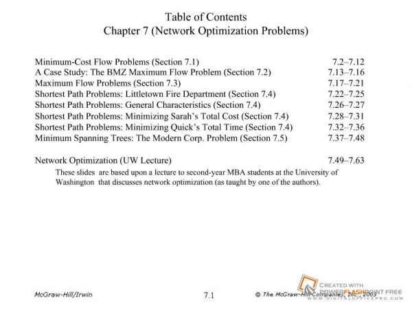
Slide 1:Table of ContentsChapter 7 (Network Optimization Problems)

Minimum-Cost Flow Problems (Section 7.1) 7.2�7.12 A Case Study: The BMZ Maximum Flow Problem (Section 7.2) 7.13�7.16 Maximum Flow Problems (Section 7.3) 7.17�7.21 Shortest Path Problems: Littletown Fire Department (Section 7.4) 7.22�7.25 Shortest Path Problems: General Characteristics (Section 7.4) 7.26�7.27 Shortest Path Problems: Minimizing Sarah�s Total Cost (Section 7.4) 7.28�7.31 Shortest Path Problems: Minimizing Quick�s Total Time (Section 7.4) 7.32�7.36 Minimum Spanning Trees: The Modern Corp. Problem (Section 7.5) 7.37�7.48 Network Optimization (UW Lecture) 7.49�7.63 These slides are based upon a lecture to second-year MBA students at the University of Washington that discusses network optimization (as taught by one of the authors).

Slide 2:Distribution Unlimited Co. Problem

The Distribution Unlimited Co. has two factories producing a product that needs to be shipped to two warehouses Factory 1 produces 80 units. Factory 2 produces 70 units. Warehouse 1 needs 60 units. Warehouse 2 needs 90 units. There are rail links directly from Factory 1 to Warehouse 1 and Factory 2 to Warehouse 2. Independent truckers are available to ship up to 50 units from each factory to the distribution center, and then 50 units from the distribution center to each warehouse. Question: How many units (truckloads) should be shipped along each shipping lane?

Slide 3:The Distribution Network

Figure 7.1 The distribution network for the Distribution Unlimited Co. problem, where each feasible shipping lane is represented by an arrow.Figure 7.1 The distribution network for the Distribution Unlimited Co. problem, where each feasible shipping lane is represented by an arrow.

Slide 4:Data for Distribution Network

Figure 7.2 The data for the distribution network for the Distribution Unlimited Co. problem.Figure 7.2 The data for the distribution network for the Distribution Unlimited Co. problem.

Slide 5:A Network Model

Figure 7.3 A network model for the Distribution Unlimited Co. problem as a minimum-cost flow problem.Figure 7.3 A network model for the Distribution Unlimited Co. problem as a minimum-cost flow problem.

Slide 6:The Optimal Solution

Figure 7.4 The optimal solution for the Distribution Unlimited Co. problem, where the shipping amounts are shown in parentheses over the arrows.Figure 7.4 The optimal solution for the Distribution Unlimited Co. problem, where the shipping amounts are shown in parentheses over the arrows.

Slide 7:Terminology for Minimum-Cost Flow Problems

The model for any minimum-cost flow problem is represented by a network with flow passing through it. The circles in the network are called nodes. Each node where the net amount of flow generated (outflow minus inflow) is a fixed positive number is a supply node. Each node where the net amount of flow generated is a fixed negative number is a demand node. Any node where the net amount of flow generated is fixed at zero is a transshipment node. Having the amount of flow out of the node equal the amount of flow into the node is referred to as conservation of flow. The arrows in the network are called arcs. The maximum amount of flow allowed through an arc is referred to as the capacity of that arc.

Slide 8:Assumptions of a Minimum-Cost Flow Problem

At least one of the nodes is a supply node. At least one of the other nodes is a demand node. All the remaining nodes are transshipment nodes. Flow through an arc is only allowed in the direction indicated by the arrowhead, where the maximum amount of flow is given by the capacity of that arc. (If flow can occur in both directions, this would be represented by a pair of arcs pointing in opposite directions.) The network has enough arcs with sufficient capacity to enable all the flow generated at the supply nodes to reach all the demand nodes. The cost of the flow through each arc is proportional to the amount of that flow, where the cost per unit flow is known. The objective is to minimize the total cost of sending the available supply through the network to satisfy the given demand. (An alternative objective is to maximize the total profit from doing this.)

Slide 9:Properties of Minimum-Cost Flow Problems

The Feasible Solutions Property: Under the previous assumptions, a minimum-cost flow problem will have feasible solutions if and only if the sum of the supplies from its supply nodes equals the sum of the demands at its demand nodes. The Integer Solutions Property: As long as all the supplies, demands, and arc capacities have integer values, any minimum-cost flow problem with feasible solutions is guaranteed to have an optimal solution with integer values for all its flow quantities.

Slide 10:Spreadsheet Model

Figure 7.5 A spreadsheet model for the Distribution Unlimited Co. minimum-cost flow problem, including the target cell Total Cost (D11). The changing cells Ship (D4:D9) show the optimal shipping quantities through the distribution network obtained by the Solver.Figure 7.5 A spreadsheet model for the Distribution Unlimited Co. minimum-cost flow problem, including the target cell Total Cost (D11). The changing cells Ship (D4:D9) show the optimal shipping quantities through the distribution network obtained by the Solver.

Slide 11:The SUMIF Function

The SUMIF formula can be used to simplify the node flow constraints. =SUMIF(Range A, x, Range B) For each quantity in (Range A) that equals x, SUMIF sums the corresponding entries in (Range B). The net outflow (flow out � flow in) from node x is then =SUMIF(�From labels�, x, �Flow�) � SUMIF(�To labels�, x, �Flow�)

Slide 12:Typical Applications of Minimum-Cost Flow Problems

Table 7.1 Typical kinds of applications of minimum-cost flow problems.Table 7.1 Typical kinds of applications of minimum-cost flow problems.

Slide 13:The BMZ Maximum Flow Problem

The BMZ Company is a European manufacturer of luxury automobiles. Its exports to the United States are particularly important. BMZ cars are becoming especially popular in California, so it is particularly important to keep the Los Angeles center well supplied with replacement parts for repairing these cars. BMZ needs to execute a plan quickly for shipping as much as possible from the main factory in Stuttgart, Germany to the distribution center in Los Angeles over the next month. The limiting factor on how much can be shipped is the limited capacity of the company�s distribution network. Question: How many units should be sent through each shipping lane to maximize the total units flowing from Stuttgart to Los Angeles?

Slide 14:The BMZ Distribution Network

Figure 7.6 The BMZ Co. distribution network from its main factory in Stuttgart, Germany, to a distribution center in Los Angeles.Figure 7.6 The BMZ Co. distribution network from its main factory in Stuttgart, Germany, to a distribution center in Los Angeles.

Slide 15:A Network Model for BMZ

Figure 7.7 A network model for the BMZ Co. problem as a maximum flow problem, where the number in square brackets below each arc is the capacity of that arc.Figure 7.7 A network model for the BMZ Co. problem as a maximum flow problem, where the number in square brackets below each arc is the capacity of that arc.

Slide 16:Spreadsheet Model for BMZ

Slide 17:Assumptions of Maximum Flow Problems

All flow through the network originates at one node, called the source, and terminates at one other node, called the sink. (The source and sink in the BMZ problem are the factory and the distribution center, respectively.) All the remaining nodes are transshipment nodes. Flow through an arc is only allowed in the direction indicated by the arrowhead, where the maximum amount of flow is given by the capacity of that arc. At the source, all arcs point away from the node. At the sink, all arcs point into the node. The objective is to maximize the total amount of flow from the source to the sink. This amount is measured in either of two equivalent ways, namely, either the amount leaving the source or the amount entering the sink.

Slide 18:BMZ with Multiple Supply and Demand Points

BMZ has a second, smaller factory in Berlin. The distribution center in Seattle has the capability of supplying parts to the customers of the distribution center in Los Angeles when shortages occur at the latter center. Question: How many units should be sent through each shipping lane to maximize the total units flowing from Stuttgart and Berlin to Los Angeles and Seattle?

Slide 19:Network Model for The Expanded BMZ Problem

Figure 7.9 A network model for the expanded BMZ Co. problem as a maximum flow problem, where the number in square brackets below each arc is the capacity of that arc.Figure 7.9 A network model for the expanded BMZ Co. problem as a maximum flow problem, where the number in square brackets below each arc is the capacity of that arc.

Slide 20:Spreadsheet Model

Figure 7.10 A spreadsheet model for the expanded BMZ Co. problem as a variant of a maximum flow problem with sources in both Stuttgart and Berlin and sinks in both Los Angeles and Seattle. Using the target cell Maximum Flow (D21) to maximize the total flow from the two sources to the two sinks, the Solver yields the optimal shipping plan shown in the changing cells Ship (D4:D19).Figure 7.10 A spreadsheet model for the expanded BMZ Co. problem as a variant of a maximum flow problem with sources in both Stuttgart and Berlin and sinks in both Los Angeles and Seattle. Using the target cell Maximum Flow (D21) to maximize the total flow from the two sources to the two sinks, the Solver yields the optimal shipping plan shown in the changing cells Ship (D4:D19).

Slide 21:Some Applications of Maximum Flow Problems

Maximize the flow through a distribution network, as for BMZ. Maximize the flow through a company�s supply network from its vendors to its processing facilities. Maximize the flow of oil through a system of pipelines. Maximize the flow of water through a system of aqueducts. Maximize the flow of vehicles through a transportation network.

Slide 22:Littletown Fire Department

Littletown is a small town in a rural area. Its fire department serves a relatively large geographical area that includes many farming communities. Since there are numerous roads throughout the area, many possible routes may be available for traveling to any given farming community. Question: Which route from the fire station to a certain farming community minimizes the total number of miles?

Slide 23:The Littletown Road System

Figure 7.11 The road system between the Littletown Fire Station and a certain farming community, where A, B, � , H are junctions and the number next to each road shows its distance in miles.Figure 7.11 The road system between the Littletown Fire Station and a certain farming community, where A, B, � , H are junctions and the number next to each road shows its distance in miles.

Slide 24:The Network Representation

Figure 7.12 The network representation of Figure 7.11 as a shortest path problem.Figure 7.12 The network representation of Figure 7.11 as a shortest path problem.

Slide 25:Spreadsheet Model

Figure 7.13 A spreadsheet model for the Littletown Fire Department shortest path problem, including the target cell Total Distance (D29). The values of 1 in the changing cells On Route (D4:D27) reveal the optimal solution obtained by the Solver for the shortest path (19 miles) from the fire station to the farming community.Figure 7.13 A spreadsheet model for the Littletown Fire Department shortest path problem, including the target cell Total Distance (D29). The values of 1 in the changing cells On Route (D4:D27) reveal the optimal solution obtained by the Solver for the shortest path (19 miles) from the fire station to the farming community.

Slide 26:Assumptions of a Shortest Path Problem

You need to choose a path through the network that starts at a certain node, called the origin, and ends at another certain node, called the destination. The lines connecting certain pairs of nodes commonly are links (which allow travel in either direction), although arcs (which only permit travel in one direction) also are allowed. Associated with each link (or arc) is a nonnegative number called its length. (Be aware that the drawing of each link in the network typically makes no effort to show its true length other than giving the correct number next to the link.) The objective is to find the shortest path (the path with the minimum total length) from the origin to the destination.

Slide 27:Applications of Shortest Path Problems

Minimize the total distance traveled. Minimize the total cost of a sequence of activities. Minimize the total time of a sequence of activities.

Slide 28:Minimizing Total Cost: Sarah�s Car Fund

Sarah has just graduated from high school. As a graduation present, her parents have given her a car fund of $21,000 to help purchase and maintain a three-year-old used car for college. Since operating and maintenance costs go up rapidly as the car ages, Sarah may trade in her car on another three-year-old car one or more times during the next three summers if it will minimize her total net cost. (At the end of the four years of college, her parents will trade in the current used car on a new car for Sarah.) Question: When should Sarah trade in her car (if at all) during the next three summers?

Slide 29:Sarah�s Cost Data

Table 7.2 Sarah�s data each time she purchases a three-year-old carTable 7.2 Sarah�s data each time she purchases a three-year-old car

Slide 30:Shortest Path Formulation

Figure 7.14 Formulation of the problem of when Sarah should trade in her car as a shortest path problem. The node labels measure the number of years from now. Each arc represents purchasing a car and then trading it in later.Figure 7.14 Formulation of the problem of when Sarah should trade in her car as a shortest path problem. The node labels measure the number of years from now. Each arc represents purchasing a car and then trading it in later.

Slide 31:Spreadsheet Model

Figure 7.15 A spreadsheet model that formulates Sarah�s problem as a shortest path problem where the objective is to minimize the total cost instead of the total distance. After applying the Solver, the values of 1 in the changing cells On Route (D12:D21) identify the shortest (least expensive) path for scheduling trade-ins.Figure 7.15 A spreadsheet model that formulates Sarah�s problem as a shortest path problem where the objective is to minimize the total cost instead of the total distance. After applying the Solver, the values of 1 in the changing cells On Route (D12:D21) identify the shortest (least expensive) path for scheduling trade-ins.

Slide 32:Minimizing Total Time: Quick Company

The Quick Company has learned that a competitor is planning to come out with a new kind of product with great sales potential. Quick has been working on a similar product that had been scheduled to come to market in 20 months. Quick�s management wishes to rush the product out to meet the competition. Each of four remaining phases can be conducted at a normal pace, at a priority pace, or at crash level to expedite completion. However, the normal pace has been ruled out as too slow for the last three phases. $30 million is available for all four phases. Question: At what pace should each of the four phases be conducted?

Slide 33:Time and Cost of the Four Phases

Table 7.3 Time required for the phases of preparing Quick Company�s new product. Table 7.4 Cost for the phases of preparing Quick Company�s new product.Table 7.3 Time required for the phases of preparing Quick Company�s new product. Table 7.4 Cost for the phases of preparing Quick Company�s new product.

Slide 34:Shortest Path Formulation

Figure 7.16 Formulation of the Quick Company problem as a shortest path problem. Except for the dummy destination, the arc labels indicate, first, the number of phases completed and, second, the amount of money left (in millions of dollars) for the remaining phases. Each arc length gives the time (in months) to perform that phase.Figure 7.16 Formulation of the Quick Company problem as a shortest path problem. Except for the dummy destination, the arc labels indicate, first, the number of phases completed and, second, the amount of money left (in millions of dollars) for the remaining phases. Each arc length gives the time (in months) to perform that phase.

Slide 35:Spreadsheet Model

Figure 7.17 A spreadsheet model that formulates the Quick Company problem as a shortest path problem where the objective is to minimize the total time instead of the total distance, so the target cell is Total Time (D32). The values of 1 in the changing cells On Route (D4:D30) reveal the shortest (quickest) path obtained by the Solver.Figure 7.17 A spreadsheet model that formulates the Quick Company problem as a shortest path problem where the objective is to minimize the total time instead of the total distance, so the target cell is Total Time (D32). The values of 1 in the changing cells On Route (D4:D30) reveal the shortest (quickest) path obtained by the Solver.

Slide 36:The Optimal Solution

Table 7.5 The optimal solution obtained by the Excel Solver for Quick Company�s shortest path problem.Table 7.5 The optimal solution obtained by the Excel Solver for Quick Company�s shortest path problem.

Slide 37:Minimum Spanning Trees:The Modern Corp. Problem

Modern Corporation has decided to have a state-of-the-art fiber-optic network installed to provide high-speed communication (data, voice, and video) between its major centers. Any pair of centers do not need to have a cable directly connecting them in order to take advantage of the technology. All that is necessary is to have a series of cables that connect the centers. Question: Which cables should be installed to provide high-speed communications between every pair of centers.

Slide 38:Modern Corporation�s Major Centers

Figure 7.18 A display of Modern Corporation�s major centers (the nodes), the possible locations for fiber-optic cables (the dashed lines), and the cost in millions of dollars for those cables (the numbers).Figure 7.18 A display of Modern Corporation�s major centers (the nodes), the possible locations for fiber-optic cables (the dashed lines), and the cost in millions of dollars for those cables (the numbers).

Slide 39:The Optimal Solution

Figure 7.19 The fiber-optic network that provides the optimal solution for Modern Corp.�s minimum-spanning-tree problem.Figure 7.19 The fiber-optic network that provides the optimal solution for Modern Corp.�s minimum-spanning-tree problem.

Slide 40:Assumptions of a Minimum-Spanning Tree Problem

You are given the nodes of a network but not the links. Instead, you are given the potential links and the positive cost (or a similar measure) for each if it is inserted into the network. You wish to design the network by inserting enough links to satisfy the requirement that there be a path between every pair of nodes. The objective is to satisfy this requirement in a way that minimizes the total cost of doing so.

Slide 41:Algorithm for a Minimum-Spanning-Tree Problem

Choice of the first link: Select the cheapest potential link. Choice of the next link: Select the cheapest potential link between a node that already is touched by a link and a node that does not yet have such a link. Repeat step 2 over and over until every node is touched by a link (perhaps more than one). At that point, an optimal solution (a minimum spanning tree) has been obtained. (Ties for the cheapest potential link at each step may be broken arbitrarily.)

Slide 42:Application of Algorithm to Modern Corp.: First Link

C-D and E-F are tied for the cheapest link. Arbitrarily choose C-D.C-D and E-F are tied for the cheapest link. Arbitrarily choose C-D.

Slide 43:Application of Algorithm to Modern Corp.: Second Link

B-C is the cheapest link that connects a node to the existing network (C-D).B-C is the cheapest link that connects a node to the existing network (C-D).

Slide 44:Application of Algorithm to Modern Corp.: Third Link

A-B is the cheapest link that connects a node to the existing network (B-C-D).A-B is the cheapest link that connects a node to the existing network (B-C-D).

Slide 45:Application of Algorithm to Modern Corp.: Fourth Link

C-F is the cheapest link that connects a node to the existing network (A-B-C-D).C-F is the cheapest link that connects a node to the existing network (A-B-C-D).

Slide 46:Application of Algorithm to Modern Corp.: Fifth Link

E-F is the cheapest link that connects a node to the existing network.E-F is the cheapest link that connects a node to the existing network.

Slide 47:Application of Algorithm to Modern Corp.: Final Link

E-G is the cheapest link that connects a node to the existing network.E-G is the cheapest link that connects a node to the existing network.

Slide 48:Applications of Minimum-Spanning-Tree Problems

Design of telecommunication networks (computer networks, lease-line telephone networks, cable television networks, etc.) Design of a lightly-used transportation network to minimize the total cost of providing the links (rail lines, roads, etc.) Design of a network of high-voltage electrical power transmission lines. Design of a network of wiring on electrical equipment (e.g., a digital computer system) to minimize the total length of the wire. Design of a network of pipelines to connect a number of locations.

Slide 49:Network Optimization Problems

Many optimization problems can be represented by a graphical network representation. Examples: Distribution problems Routing problems Maximum flow problems Designing computer / phone / road networks Equipment replacement Slides 7.49-7.63 are based upon a lecture from a 2nd-year MBA elective course �Modeling with Spreadsheets� at the University of Washington (as taught by one of the authors). The lecture covers network optimization problems. Slides 7.49-7.63 are based upon a lecture from a 2nd-year MBA elective course �Modeling with Spreadsheets� at the University of Washington (as taught by one of the authors). The lecture covers network optimization problems.

Slide 50:Components of a Minimum-Cost-Flow Model

Nodes can represent a location, point in time, or state supply node (flow is generated) demand node (flow is consumed) transshipment node (flow in = flow out) Arcs can represent potential flow (e.g., a shipping lane) or a transition from state to state. directional (one-way) if both ways, use two arcs cost (assumed proportional to flow) may have capacity

Slide 51:Minimum-Cost-Flow Model

Objective: Minimize the total cost of all flow, while sending supply through the network to satisfy demand. Integer Solutions Property: If supplies, demands, and arc capacities are integer, then the optimal flow will also be integer. Network Simplex Method: A streamlined version of the simplex method. extremely efficient computer software may have graphical interface (with nodes and arcs) Excel uses the standard simplex method. However, the minimum-cost-flow model is a useful tool for modeling a problem: visual intuitive easy to set up transforms easily to a spreadsheet model

Slide 52:Multi-Echelon Distribution

Consider a multi-echelon distribution problem. Product must be distributed from a pair of factories to three warehouses. Product is then shipped to five distribution centers. A private trucking fleet is used for all shipping. Some shipping lanes are currently capacitated due to a limited number of trucks. Question: How many units should be shipped along each shipping lane?

Slide 53:Spreadsheet Model

To discuss: May also lay out in table form (i.e., as a transportation problem) This network representation is more efficient if the network is sparse.To discuss: May also lay out in table form (i.e., as a transportation problem) This network representation is more efficient if the network is sparse.

Slide 54:The SUMIF Function

The SUMIF formula can be used to simplify the node flow constraints. =SUMIF(Range A, x, Range B) For each quantity in (Range A) that equals x, SUMIF sums the corresponding entries in (Range B). The net outflow (flow out � flow in) from node x is then =SUMIF(�From labels�, x, �Flow�) � SUMIF(�To labels�, x, �Flow�) Normally Solver does not like IF (or SUMIF) statements in a linear model. It�s okay here because the logic of the SUMIF statement does not involve changing cells, only data cells. In effect, all of the SUMIF statement logic could be evaluated before even evaluating the changing cells. It is just an easier way to enter a whole set of net flow calculations, since the formula need only be entered once and then copied to the other rows. This also reduces the chance for error.Normally Solver does not like IF (or SUMIF) statements in a linear model. It�s okay here because the logic of the SUMIF statement does not involve changing cells, only data cells. In effect, all of the SUMIF statement logic could be evaluated before even evaluating the changing cells. It is just an easier way to enter a whole set of net flow calculations, since the formula need only be entered once and then copied to the other rows. This also reduces the chance for error.

Slide 55:Spreadsheet Model using SUMIF

While the SUMIF function looks more complicated, it is actually quicker and easier to enter than the previous way (entering the formula by hand for each row). The formula can be entered once, and then copied to all of the other rows. This reduces the chance for an error, which is almost inevitable when entering each formula by hand.While the SUMIF function looks more complicated, it is actually quicker and easier to enter than the previous way (entering the formula by hand for each row). The formula can be entered once, and then copied to all of the other rows. This reduces the chance for an error, which is almost inevitable when entering each formula by hand.

Slide 56:The Minimum-Cost-Flow Model is an LP

Any minimum cost flow model consists of a set of nodes: Supply node(s), with supply si Demand node(s), with demand di Transshipment nodes A set of arcs from node i to node j with cost cij some with limited capacity kij LP Formulation: Let xij = flow from i to jMinimize Cost = ? ij cij xijsubject to Flow: ?all j flowing out of i xij � ?all j flowing into i xji = (si, di, or 0) Capacity: xij = kijand xij = 0.

Slide 57:Maximum Flow Problem

An oil company has the following pipeline network, where each pipeline is labeled with its maximum flow rate (in thousands of gallons per hour). Question: What is the maximum possible flow rate from A to G? Network model: Cost is ignored. Net flow = 0 at transshipment nodes Leave starting / ending nodes unconstrained Maximize supply at start nodeNetwork model: Cost is ignored. Net flow = 0 at transshipment nodes Leave starting / ending nodes unconstrained Maximize supply at start node

Slide 58:Spreadsheet Model

Slide 59:Shortest Path Problem

The travel times along various routes in the Pacific Northwest is shown below. Question: What is the quickest route from Seattle to Denver? Network model: No capacity constraints Cost = driving time (or distance or cost) Supply = 1 at Start Demand = 1 at End Minimize Cost (Time)Network model: No capacity constraints Cost = driving time (or distance or cost) Supply = 1 at Start Demand = 1 at End Minimize Cost (Time)

Slide 60:Spreadsheet Model

Route = (where flow = 1).Route = (where flow = 1).

Slide 61:Equipment Replacement

A production department needs to purchase a new machine. As the machine ages, it requires additional maintenance and also has a higher defect rate. The production department plans to replace the machine every few years. The purchase price of a new machine is $10,000. The maintenance cost and cost of defective product is given below. A used machine has no resale value. Question: What is the best replacement policy over the next five years? Network model: Node = year Arc = action (length of time to keep)Network model: Node = year Arc = action (length of time to keep)

Slide 62:Spreadsheet Solution

Slide 63:Planning Vehicle Replacement at Phillips Petroleum

Phillips Petroleum had a fleet of 1,500 cars and 3,800 trucks. Modeled replacement strategy as shortest path model (20-year time horizon)�solved model once for each class of vehicle. Could keep, purchase (replace), or lease, at 3-month intervals. Costs considered included: Maintenance and operating costs (fuel, oil, repair), Leasing cost for leased vehicles, Purchasing cost for purchased vehicles, State license fees and road taxes, Tax effects (investment tax credits, depreciation) First used to make lease-or-buy decision, then vehicle-replacement strategy, and more recently for other equipment (non-vehicle). For more details, see Waddell (1983) Jul-Aug Interfaces article, �A Model for Equipment Replacement Decisions and Policies�, downloadable at www.mhhe.com/hillier2e/articles.