Download
1 / 38
460 likes | 1.31k Views
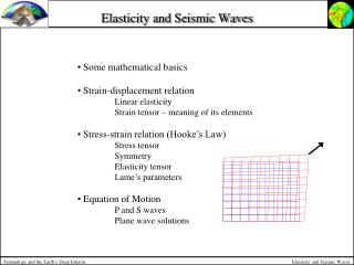
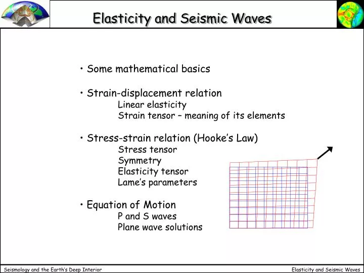
Elasticity and Seismic Waves. Some mathematical basics Strain-displacement relation Linear elasticity Strain tensor – meaning of its elements Stress-strain relation (Hooke’s Law) Stress tensor Symmetry Elasticity tensor Lame’s parameters Equation of Motion P and S waves

E N D
Elasticity and Seismic Waves • Some mathematical basics • Strain-displacement relation • Linear elasticity • Strain tensor – meaning of its elements • Stress-strain relation (Hooke’s Law) • Stress tensor • Symmetry • Elasticity tensor • Lame’s parameters • Equation of Motion • P and S waves • Plane wave solutions
Breaking Linear deformation Stable slip Stick slip Stress-strain regimes • Linear elasticity (teleseismic waves) • rupture, breaking • stable slip (aseismic) • stick-slip (with sudden ruptures) Stress Deformation
Linear and non-linear stress and strain Linear stress-strain Stress vs. strain for a loading cycle with rock that breaks. For wave propagation problems assuming linear elasticity is usually sufficient.
Principal stress, hydrostatic stress Horizontal stresses are influenced by tectonic forces (regional and local). This implies that usually there are two uneven horizontal principal stress directions. Example: Cologne Basin When all three orthogonal principal stresses are equal we speak of hydrostatic stress.
Elasticity Theory A time-dependent perturbation of an elastic medium (e.g. a rupture, an earthquake, a meteorite impact, a nuclear explosion etc.) generates elastic waves emanating from the source region. These disturbances produce local changes in stress and strain. To understand the propagation of elastic waves we need to describe kinematically the deformation of our medium and the resulting forces (stress). The relation between deformation and stress is governed by elastic constants. The time-dependence of these disturbances will lead us to the elastic wave equation as a consequence of conservation of energy and momentum.
Some mathematical basics - Vectors The mathematical description of deformation processes heavily relies on vector analysis. We therefore review the fundamental concepts of vectors and tensors. Usually vectors are written in boldface type, x is a scalar but y is a vector, yi are the scalar components of a vector Scalar or Dot Product b c=a+b b=c-a a=c-b a q c
y bxc a c x b z Vectors – Triple Product The vector cross product is defined as: The triple scalar product is defined as which is a scalar and represents the volume of the parallelepiped defined by a,b, and c. It is also calculated like a determinant:
Vectors – Gradient Assume that we have a scalar field F(x), we want to know how it changes with respect to the coordinate axes, this leads to a vector called the gradient of F and With the nabla operator The gradient is a vector that points in the direction of maximum rate of change of the scalar function F(x). What happens if we have a vector field?
Vectors – Divergence + Curl The divergence is the scalar product of the nabla operator with a vector field V(x). The divergence of a vector field is a scalar! Physically the divergence can be interpreted as the net flow out of a volume (or change in volume). E.g. the divergence of the seismic wavefield corresponds to compressional waves. The curl is the vector product of the nabla operator with a vector field V(x). The curl of a vector field is a vector! The curl of a vector field represents the rotational part of that field (e.g. shear waves in a seismic wavefield)
Vectors – Gauss’ Theorem Gauss’ theorem is a relation between a volume integral over the divergence of a vector field F and a surface integral over the values of the field at its surface S: dS=njdS V S … it is one of the most widely used relations in mathematical physics. The physical interpretation is again that the value of this integral can be considered the net flow out of volume V.
Q1 y P1 x u v u Q0 x Deformation Let us consider a point P0 at position r relative to some fixed origin and a second point Q0 displaced from P0 by dx Unstrained state: Relative position of point P0 w.r.t. Q0 is x. Strained state: Relative position of point P0 has been displaced a distance u to P1 and point Q0 a distance v to Q1. Relative positive of point P1 w.r.t. Q1 is y= x+ u. The change in relative position between Q and P is just u. y P0 r x
Q1 y P1 x u v u P0 Q0 x Linear Elasticity The relative displacement in the unstrained state is u(r). The relative displacement in the strained state is v=u(r+ x). So finally we arrive at expressing the relative displacement due to strain: u=u(r+ x)-u(r) We now apply Taylor’s theorem in 3-D to arrive at: What does this equation mean?
Q1 y P1 x u v u P0 Q0 x Linear Elasticity – symmetric part The partial derivatives of the vector components represent a second-rank tensor which can be resolved into a symmetric and anti-symmetric part: • antisymmetric • pure rotation • symmetric • deformation
Q1 y P1 x u v u P0 Q0 x Linear Elasticity – deformation tensor The symmetric part is called the deformation tensor and describes the relation between deformation and displacement in linear elasticity. In 2-D this tensor looks like
Deformation tensor – its elements Through eigenvector analysis the meaning of the elements of the deformation tensor can be clarified: The deformation tensor assigns each point – represented by position vector y a new position with vector u (summation over repeated indices applies): The eigenvectors of the deformation tensor are those y’s for which the tensor is a scalar, the eigenvalues l: The eigenvalues l can be obtained solving the system:
Deformation tensor – its elements Thus ... in other words ... the eigenvalues are the relative change of length along the three coordinate axes shear angle In arbitrary coordinates the diagonal elements are the relative change of length along the coordinate axes and the off-diagonal elements are the infinitesimal shear angles.
Deformation tensor – trace The trace of a tensor is defined as the sum over the diagonal elements. Thus: This trace is linked to the volumetric change after deformation. Before deformation the volume was V0. . Because the diagonal elements are the relative change of lengths along each direction, the new volume after deformation is ... and neglecting higher-order terms ...
Deformation tensor – applications The fact that we have linearised the strain-displacement relation is quite severe. It means that the elements of the strain tensor should be <<1. Is this the case in seismology? Let’s consider an example. The 1999 Taiwan earthquake (M=7.6) was recorded in FFB. The maximum ground displacement was 1.5mm measured for surface waves of approx. 30s period. Let us assume a phase velocity of 5km/s. How big is the strain at the Earth’s surface, give an estimate ! The answer is that e would be on the order of 10-7 <<1. This is typical for global seismology if we are far away from the source, so that the assumption of infinitesimal displacements is acceptable. For displacements closer to the source this assumption is not valid. There we need a finite strain theory. Strong motion seismology is an own field in seismology concentrating on effects close to the seismic source.
Borehole breakout Source: www.fracom.fi
tk t1 t2 t3 Stress - traction In an elastic body there are restoring forces if deformation takes place. These forces can be seen as acting on planes inside the body. Forces divided by an areas are called stresses. In order for the deformed body to remain deformed these forces have to compensate each other. We will see that the relationship between the stress and the deformation (strain) is linear and can be described by tensors. The tractions tk along axis k are ... and along an arbitrary direction ... which – using the summation convention yields ..
Stress tensor 3 ... in components we can write this as 2 where ij ist the stress tensor and nj is a surface normal. The stress tensor describes the forces acting on planes within a body. Due to the symmetry condition 21 22 23 1 there are only six independent elements. The vector normal to the corresponding surface The direction of the force vector acting on that surface
Stress equilibrium If a body is in equilibrium the internal forces and the forces acting on its surface have to vanish as well as the sum over the angular momentum From the second equation the symmetry of the stress tensor can be derived. Using Gauss’ law the first equation yields
Stress-strain relation The relation between stress and strain in general is described by the tensor of elastic constants cijkl Generalised Hooke’s Law From the symmetry of the stress and strain tensor and a thermodynamic condition if follows that the maximum number if independent constants of cijkl is 21. In an isotropic body, where the properties do not depend on direction the relation reduces to Hooke’s Law where l and m are the Lame parameters, q is the dilatation and dij is the Kronecker delta.
Stress-strain relation The complete stress tensor looks like There are several other possibilities to describe elasticity: E elasticity, s Poisson’s ratio, k bulk modulus For Poisson’s ratio we have 0<s<0.5. A useful approximation is l=m, then s=0.25. For fluids s=0.5 (m=0).
Stress-strain - significance As in the case of deformation the stress-strain relation can be interpreted in simple geometric terms: u u l l g Remember that these relations are a generalization of Hooke’s Law: F= D s D being the spring constant and s the elongation.
Elastic anisotropy What is seismic anisotropy? • Seismic wave propagation in anisotropic media is quite different from isotropic media: • There are in general 21 independent elastic constants (instead of 2 • in the isotropic case) • there is shear wave splitting (analogous to optical birefringence) • waves travel at different speeds depending in the direction of • propagation • The polarization of compressional and shear waves may not be • perpendicular or parallel to the wavefront, resp.
Anisotropic wave fronts From Brietzke, Diplomarbeit
Elastic anisotropy - Data • Azimuthal variation of velocities in the upper mantle observed under the pacific ocean. • What are possible causes for this anisotropy? • Aligned crystals • Flow processes
Elastic anisotropy - olivine Explanation of observed effects with olivine crystals aligned along the direction of flow in the upper mantle
Elastic anisotropy – applications • Crack-induced anisotropy • Pore space aligns itself in the stress field. Cracks are aligned perpendicular to the minimum compressive stress. The orientation of cracks is of enormous interest to reservoir engineers! • Changes in the stress field may alter the density and orientation of cracks. Could time-dependent changes allow prediction of ruptures, etc. ? • SKS - Splitting • Could anisotropy help in understanding mantle flow processes?
Equations of motion We now have a complete description of the forces acting within an elastic body. Adding the inertia forces with opposite sign leads us from to the equations of motion for dynamic elasticity
Summary: Elasticity - Stress Seismic wave propagation can in most cases be described by linear elasticity. The deformationof a medium is described by the symmetric elasticity tensor. The internal forces acting on virtual planes within a medium are described by the symmetric stress tensor. The stress and strain are linked by the material parameters (like spring constants) through the generalised Hooke’s Law. In isotropic media there are only two elastic constants, the Lame parameters. In anisotropic media the wave speeds depend on direction and there are a maximum of 21 independant elastic constants. The most common anisotropic symmetry systems are hexagonal (5) and orthorhombic (9 independent constants).