Download
1 / 46
460 likes | 877 Views
An Introduction to Random Number Generators and Monte Carlo Methods. Josh Gilkerson Wei Li David Owen. Random Number Generators. Uses for Random Numbers. Monte Carlo Simulations Generation of Cryptographic Keys Evolutionary Algorithms Many Combinatorial Optimization Algorithms.

E N D
An Introduction to Random Number Generators and Monte Carlo Methods Josh Gilkerson Wei Li David Owen
Uses for Random Numbers • Monte Carlo Simulations • Generation of Cryptographic Keys • Evolutionary Algorithms • Many Combinatorial Optimization Algorithms
Two Types of Random Numbers • Pseudorandom numbers are numbers that appear random, but are obtained in a deterministic, repeatable, and predictable manner. • True random numbers are generated in non-deterministic ways. They are not predictable. They are not repeatable.
True Random Generators • Use one of several sources of randomness • decay times of radioactive material • electrical noise from a resistor or semiconductor • radio channel or audible noise • keyboard timings • some are better than others • usually slower than PRNGs
RNG And Random Machines • It is not viable to generate a true random number using computers since they are deterministic. However, we can generate a good enough random numbers that have properties close to true random numbers. • The first machine used to produce a table of 100,000 random digits was done by M. G. Kendall and B. Babington-Smith in 1939. • RAND Corporation in 1955 released a table of a million random digits. • ERNIE is a random number generator machine used to pick the winning numbers in the British Premium Bonds lottery.
Desirable Properties of PRNGs • Uniform • Lengthy period • Serially uncorrelated • Fast
Problems With PRNG • It is very difficult to pin point the problem with random number generators when they arise. Usually, the programmers would need to replace the whole random number generator with a better ones. • With small test cases, problems rarely arises. However, when it gets to large scale random number generations (possibly in millions or even billions of numbers) the problem could be apparent. This makes debugging difficult. • In large-scale computing problems, one might need to use a parallel algorithm. The effect is that, sometimes it is not possible to duplicate the simulation exactly.
Linear Congruential Generator(LCG) • Most common • Maximum period of 2n for n-bit numbers • Xn+1=( aXn + c ) mod m • a,c,m are constants • X0 is the seed
Advantages of LCG • Most common • Very easily implemented • Fast and small (remember only last number) • Easily parallelized • N processes 1 ... N. • numbers for process n are Xn+iN • no more expensive than serial version.
Disadvantages of LCGs • Other generators have longer maximum periods. • Bad choices of M result in very bad sequences (primes work best, powers of 2 are fast, but not nearly as good). • Initial seed affects period. • Low order bits are not random.
Lagged Fibonacci Generators • Similar to Fibonacci Sequence • Increasingly popular • Xn = (Xn-l + Xn-k) mod m (l>k>0) • l seeds are needed • m usually a power of 2 • Maximum period of (2l-1)x2M-1 when m=2M
Add-with-carry & Subtract-with-borrow • Similar to LFG • AWC: Xn=(Xn-l+Xn-k+carry) mod m • SWB: Xn=(Xn-l-Xn-k-carry) mod m
Multiply-with-carry Generators • Similar to LCG • Xn=(aXn-1+carry) mod m
Inverse Congruential Generators • Xn=(a * ~Xn-1 + b) mod m • m should be prime • ~y is the multiplicative inverse of y in the field over {0,1,...,m-1}.
PRNG Review • This is just a short review. There are many other PRNGs. • Linear Congruential Generator • Lagged Fibonacci Generator • Add-with-carry Generator • Subtract-with-carry Generator • Multiply-with-carry Generator • Inverse Congruential Generator
Testing Randomness • Test for uniform distribution (of singletons, pairs, triples, etc) of the sequence and all subsequences. • DIEHARD - http://stat.fsu.edu/pub/diehard/ • NIST - http://csrs.nist.gov/rng
Introduction of Monte Carlo • Monte Carlo methods have been used for centuries. • However during World War II, this method was used to simulate the probabilistic issues with neutron diffusion (first real use). • Named after the capital of Monaco (one of the world’s center for gambling), due to the similarity to games of chance.
What is Monte Carlo • Non Monte Carlo methods typically involve ODE/PDE equations that describe the system. • Monte Carlo methods are stochastic techniques. • It is based on the use of random numbers and probability statistics to simulate problems. • Something can be called a Monte Carlo method if it uses random numbers to examine the problem it is solving. • First, we would need to determine the probability density function (PDF). Then perform random sampling from the PDF. We keep record of each simulation performed and tally them.
Probability Density Function • A probability density function (or probability distribution function) is a function f defined on an interval (a, b) and having the following properties:
Why use Monte Carlo • It allows us to examine complex system. And is usually easy to formulate (independent of the problem). • For example, solving equations which describe two atoms interactions. This would be doable without using Monte Carlo method. But solving the interactions for thousands of atoms using the same equations is impossible. • However, the solutions are imprecise and it can be very slow if higher precision is desired.
Components of Monte Carlo simulation • Probability distribution functions (pdf's) - the physical (or mathematical) system must be described by a set of pdf's. • Random number generator - a source of random numbers uniformly distributed on the unit interval must be available. • Sampling rule - a prescription for sampling from the specified pdf's, assuming the availability of random numbers on the unit interval, must be given. • Scoring (or tallying) - the outcomes must be accumulated into overall tallies or scores for the quantities of interest.
Components of Monte Carlo simulation (cont.) • Error estimation - an estimate of the statistical error (variance) as a function of the number of trials and other quantities must be determined. • Variance reduction techniques - methods for reducing the variance in the estimated solution to reduce the computational time for Monte Carlo simulation • Parallelization and vectorization - algorithms to allow Monte Carlo methods to be implemented efficiently on advanced computer architectures.
Monte Carlo Example (cont.) • So, we can compute PI by generating two numbers for x and y component of a simulated throw. Then we can figure out by using Pythagorean theorem if this throw is inside or outside the circle. We count this hits, and after doing this thousands of times (or more), we can get an estimate value of PI. • Accuracy of the estimate depends on the number of “throws”. An example code would be (assuming we set the radius = 1): double x = rand(); // get random # in [0, 1] for x double y = rand(); // get random # in [0, 1] for y double dist = sqrt(x*x + y*y); if (distFromOrigin(x,y) <= 1) hits++;
What MC Needs • MC methods might needs different RNG. • For example, when simulating outgoing direction for a launched particle and interactions of the particle with the medium, the following would be the desirable properties: • The attribute of each particle should be independent from each other. • The attribute of all the particles should span across the entire attribute space. I.e., as we approach infinite numbers of particles, the particles launched into a space should cover the space completely. Next slide will states the properties of the RNG needed.
What MC Needs (cont.) • Any subsequence of random numbers should not be correlated with any other subsequence of random numbers. For example, when simulating the launched particles, we should not generate geometrical patterns. • Random number repetition should occur only after a very large generation of random numbers. • The random numbers generated should be uniform. This point and the first one are loosely related. To achieve more uniformity, some correlations between random numbers must be established. • The RNG should be efficient. It should be vectorizable with low overhead. The processors in parallel systems, should not be required to talk between each other.
Appropriate PRNGs • The following are packages of available RNGs (http://www.agner.org/random/). • Uniform RNG in C++ & assembly language • Mersenne twister. • Mother-of-all. • RANROT. • In C, we can use drand48() to generate a double type of random number which is produced using 48-bit integers.
An Application of the Monte Carlo Method The Effect of Space Discretization on the Canonical Monte Carlo Simulation
Agenda • Introduction to the Monte Carlo (MC) molecular simulation • Canonical Ensemble • Importance Sampling • Simulation Process • Simulation of the equation of state of the Lennard-Jones Fluid – Continuum Model • Discretized Model • Comparison of the simulation results
Introduction • Why molecular simulation? • Help explaining experimental observations • simulate critical or extreme conditions • Guide real experiments • Purpose of this study • Long-term goal - simulation of self-assembly of surfactant solutions – fine lattice • The continuum model is not viable under the current computing power • The discretized model is at least 10 times faster compared with the continuum model • The effect of space discretization on the simulation results
Canonical Ensemble • fixed number of molecules N, fixed volume V (volume), fixed temperature T • The canonical ensemble partition function from statistical mechanics • Evaluation of observable properties A • Random sampling - brute force Monte Carlo • When estimate <f(x)> , most of the computing is wasted
Importance Sampling Change the integration variable Standard deviation Impossible to find the weight function w in multidimensional integrals
The Metropolis Method Evaluation of observable properties A Probability of finding the system in a configuration around r Randomly generate sampling points according to the probability distribution N(r)
The Detailed Balance Generate sampling points according to the probability distribution – detailed balance If α is a symmetric matrix If α is a symmetric matrix
Simulation Process • Initialize the system • Put the system in a random state • Make a trial move • Randomly make a trial move • Calculate the energy change • Reevaluate the interactions of the moved particles with its neighbors and calculate the energy change • Accept the trial move with the Metropolis scheme • Keep trying the moves until system approach equilibrium • Either monitor the total energy change, or monitor the structure formed in the simulation box • Sampling • Sample a certain property over a certain number of configurations
Continuum Model • Fixed N, V, T • Lennard-Jones potential • Intermolecular force • Virial of the system • Pressure of the system
Simulation Process Main program Monte Carlo loop Subroutine Start Start Read simulation parameters Trial move yes Satisfy Metropolis rule? Accept the trial move yes no New simulation? no Update energy and virial Initialize positions of all particles Read old configuration Sample the pressure Monte Carlo loop no End of simulation? yes Stop Stop
Parameters Modeling • Potential minimum between 2 particles • Average distance between 2 particles • Maximum displacement of a particle • Number of particles • Temperature • Density of the system
Discretized Model • Space is discretized. Particles can only move on a 3D mesh (fine lattice). • Distance between particles is a set of fixed values. • Evaluation of complex functions against distance can be precalculated. • Depends on the form the functions, the simulation can be accelerated 10-100 times move move
Conclusion • The equation of state of L-J fluid from the canonical MC simulation agrees with what reported on literature • The Discretized Model can produce results comparable to the Continuum Model • The Discretized Model can make simulations where the normal Continuum Model cannot access
RNG Resources • True Random Numbers • http://www.random.org/ • http://www.fourmilab.ch/hotbits/ • http://www.robertnz.net/hwrng.htm • http://world.std.com/~reinhold/truenoise.html • Pseudo-random Number Generators • http://random.mat.sbg.ac.at/ • http://www.math.utah.edu/~alfeld/Random/Random.html • http://www.mathcom.com/corpdir/techinfo.mdir/scifaq/q210.html • http://csep1.phy.ornl.gov/rn/rn.html • Others • ftp://ftp.isi.edu/in-notes/rfc1750.txt
Monte Carlo Method Resources • http://csep1.phy.ornl.gov/mc/mc.html • http://www.chem.unl.edu/zeng/joy/mclab/mcintro.html • http://csep1.phy.ornl.gov/rn/rn.html • http://mathworld.wolfram.com/QuasirandomSequence.html • http://www.agner.org/random/ • http://web.cz3.nus.edu.sg/~yzchen/teach/comphys/sec03.html