Download
1 / 40
400 likes | 675 Views
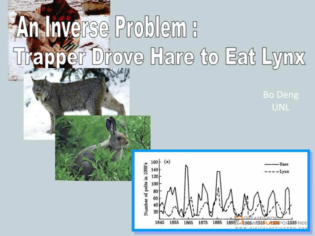
Trapper Drove Hare to Eat Lynx. An Inverse Problem : B. Blaslus, et al ... Is Hare-Lynx Dynamics Chaotic? Rate of Expansion along Time Series ~ exp(l) l = Lyapunov ...

E N D
1. title
Bo Deng UNL
B. Blaslus, et al Nature 1999 Mark O�Donoghue, et al Ecology 1998 An empirical data of a physical process P is a set of observation time and quantities: with The aim of mathematical modeling is to fit a mathematical form to the data by one of two ways: 1. phenomenologically without a conceptual model 2. mechanistically with a conceptual model We will consider only mathematical models of differential equations: with t having the same time dimension as t i j , x the state variables, and p the parameters. Inverse Problem : Let be the predicted states by the model to the observed states, Then the inverse problem is to fit the model to the data with the least dimensionless error between the predicted and the observed: The least error of the model for the process is with the minimizer being the best fit of the model to the data. The best model for the process F satisfies for all proposed models G . Gradient Search Method for Local Minimizers: In the parameter and initial state space , a search path satisfies the gradient search equation: A local minimizer is found as My belief: The fewer the local minima, the better the model. Dimensional Analysis by the Buckingham Theorem: Degree of Freedom for the Best Fit = Old Dimension � New Dimension = n � l A best fit by the dimensionless model corresponds to a (n � l )-dimensional surface of the same least error fit, i.e., best fit in general is not unique. Example: Logistic equation with Holling Type II harvesting where n = 1, m = 4, and m � n � 1 = 2. With best fit to l = 1 data set, there is zero, n � l = 0, degree of freedom.12. Basic Models
Solve it for the per-predator Predation Rate: Holling�s Type II Form (Can. Ent. 1959) where T = given time a = encounter probability rate h = handling time per prey For One Predator: X XC 1/h Prey captured during T period of time Type I Form, h = 0 Type II Form, h > 0
Dimensional Model Dimensionless Model By Method of Line Search for local extrema Left Chirality and Right Chirality : By Taylor,s expansion: Best-Fit Sensitivity : , Best-Fit Sensitivity : , All models are constructed to fail against the test of time. S. Ellner & P. Turchin Amer. Nat. 1995 Is Hare-Lynx Dynamics Chaotic? Rate of Expansion along Time Series ~ exp(l) l = Lyapunov Exponent > 0 ? Chaos N.C. Stenseth Science 1995 1844 -- 1935 Alternative Title: Holling made trappers to drive hares to eat lynx