Download
1 / 34
340 likes | 365 Views
Thermodynamics has been the foundation of many models of biological and technological<br>systems. But thermodynamics is static and is misnamed. A more suitable name is thermostatics. Thermostatics does not include time as a variable and so has no velocity, flow or friction. Indeed, as usually formulated, thermostatics does not include boundary conditions. Devices require boundary conditions to define their input and output. They usually involve flow and friction. Thermostatics is an unsuitable foundation for understanding technological and biological devices. A time<br>dependent generalization of thermostatics that might be called thermal dynamics is being<br>developed by Chun Liu and collaborators to avoid these limitations. Electrodynamics is not<br>restricted like thermostatics, but in its classical formulation involves drastic assumptions about<br>polarization and an over-approximated dielectric constant. Once the Maxwell equations are<br>rewritten without a dielectric constant, they are universal and exact. Conservation of total current, including displacement current, is a restatement of the Maxwell equations that leads to dramatic simplifications in the understanding of one dimensional systems, particularly those without branches, like the ion channel proteins of biological membranes and the two terminal devices of electronic systems. The Brownian fluctuations of concentrations and fluxes of ions become the spatially independent total current, because the displacement current acts as an unavoidable low pass filter, a consequence of the Maxwell equations for any material polarization. Electrodynamics and thermal dynamics together form a suitable foundation for models of technological and biological systems.

E N D
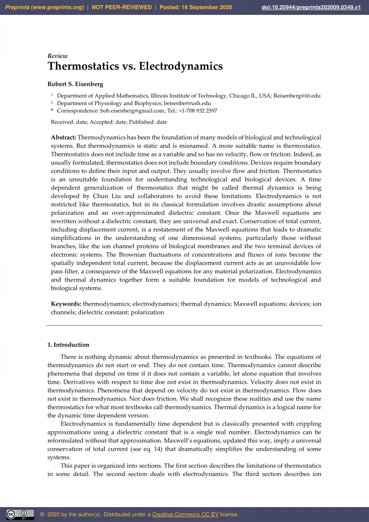
Preprints (www.preprints.org) | NOT PEER-REVIEWED | Posted: 16 September 2020 doi:10.20944/preprints202009.0349.v1 Review Thermostatics vs. Electrodynamics Robert S. Eisenberg 1 Department of Applied Mathematics, Illinois Institute of Technology, Chicago IL, USA; Reisenberg@iit.edu 2 Department of Physiology and Biophysics; beisenbe@rush.edu * Correspondence: bob.eisenberg@gmail.com; Tel.: +1-708 932 2597 Received: date; Accepted: date; Published: date Abstract: Thermodynamics has been the foundation of many models of biological and technological systems. But thermodynamics is static and is misnamed. A more suitable name is thermostatics. Thermostatics does not include time as a variable and so has no velocity, flow or friction. Indeed, as usually formulated, thermostatics does not include boundary conditions. Devices require boundary conditions to define their input and output. They usually involve flow and friction. Thermostatics is an unsuitable foundation for understanding technological and biological devices. A time dependent generalization of thermostatics that might be called thermal dynamics is being developed by Chun Liu and collaborators to avoid these limitations. Electrodynamics is not restricted like thermostatics, but in its classical formulation involves drastic assumptions about polarization and an over-approximated dielectric constant. Once the Maxwell equations are rewritten without a dielectric constant, they are universal and exact. Conservation of total current, including displacement current, is a restatement of the Maxwell equations that leads to dramatic simplifications in the understanding of one dimensional systems, particularly those without branches, like the ion channel proteins of biological membranes and the two terminal devices of electronic systems. The Brownian fluctuations of concentrations and fluxes of ions become the spatially independent total current, because the displacement current acts as an unavoidable low pass filter, a consequence of the Maxwell equations for any material polarization. Electrodynamics and thermal dynamics together form a suitable foundation for models of technological and biological systems. Keywords: thermodynamics; electrodynamics; thermal dynamics; Maxwell equations; devices; ion channels; dielectric constant; polarization 1. Introduction There is nothing dynamic about thermodynamics as presented in textbooks. The equations of thermodynamics do not start or end. They do not contain time. Thermodynamics cannot describe phenomena that depend on time if it does not contain a variable, let alone equation that involves time. Derivatives with respect to time doe not exist in thermodynamics. Velocity does not exist in thermodynamics. Phenomena that depend on velocity do not exist in thermodynamics. Flow does not exist in thermodynamics. Nor does friction. We shall recognize these realities and use the name thermostatics for what most textbooks call thermodynamics. Thermal dynamics is a logical name for the dynamic time dependent version. Electrodynamics is fundamentally time dependent but is classically presented with crippling approximations using a dielectric constant that is a single real number. Electrodynamics can be reformulated without that approximation. Maxwell’s equations, updated this way, imply a universal conservation of total current (see eq. 14) that dramatically simplifies the understanding of some systems. This paper is organized into sections. The first section describes the limitations of thermostatics in some detail. The second section deals with electrodynamics. The third section describes ion © 2020 by the author(s). Distributed under a Creative Commons CC BY license.
Preprints (www.preprints.org) | NOT PEER-REVIEWED | Posted: 16 September 2020 doi:10.20944/preprints202009.0349.v1 2 of 34 channels of biological membranes and shows the dramatics simplification electrodynamics can make. The fourth section derives the theory that provides those simplifications. The fifth section shows the general implications of electrodynamics. The sixth section and some of Discussion describes the challenges faced by molecular dynamics as it seeks to implement consistent electrodynamics on an atomic scale. The need to update the Maxwell equations is in section 7. The Discussion deals further with molecular dynamics and then shows the implications of electrodynamics for the flux coupling that is a crucial property of living systems 2. Results 2.1. Thermostatics The lack of friction in thermostatics is a serious problem because all of life and most material systems involve friction. Indeed, life and electrochemistry occur only in liquids. Liquids are called condensed phases because they have very little empty space. The average velocity of atoms is set by their temperature [1] and is roughly the speed of sound [2]. The number of collisions, defined as sudden changes in direction, is enormously high. Atoms cannot move without colliding. Only a handful of collisions is needed to convert straight line motion to the random motion we call heat. So any movement taking more than say 10−13sec in a condensed phase is likely to have significant friction. Friction is involved in the processes of biology even when they are customarily described by state models, that do not include velocity or friction as variables. State models are used throughout biology, and in much of chemistry in a liquid phase, with well defined energy states. How a system is supposed to move from one state to another without friction is not discussed. When systems do move from state to state in a condensed phase, energy is lost to heat, because they move with nonzero velocity and friction is a monotonic function of function of velocity in many cases. Thus the energy of moving from state to state is not just a function of the initial state and final state, but also depends on the path between the states. The path is unspecified and it is obvious that different states can have different profiles of velocity, and thus different amounts of friction. The energy lost to heat can have many values. In other words, it is not correct to assume that a system in a condensed phase can have energy states independent of the path to reach that state. Of course, special cases may make these frictional effects negligible, or reproducible from transition to transition, so making the usual analysis a good approximation. But approximations need to be recognized, before they can be examined. They must be examined before they can be justified. Simplicity is not a justification for ignoring a universal and essential physical process, loss of energy when movement occurs in condensed phases. Including friction in theories of motion has been a huge hurdle for applied mathematicians and has only recently been overcome. The variational calculus of Hamilton only applies to systems without friction [3-8]. The variational calculus of Rayleigh was designed to deal with friction but in an imaginary world in which only frictional forces existed [9, 10]. Rayleigh’s world was without conservative forces, presumably because he realized the difficulties of dealing with position and velocity dependent forces (i.e., conservative and dissipative forces) in one mathematical structure. Obviously, ordinary differential equations can not do the trick! Onsager tried to deal with both types of forces [11-13] but the mathematical apparatus of a variational calculus with two independent variables (position and velocity) was not available to him. It had not been invented. That “partial variational calculus”, if I can be allowed to coin a phrase in the spirit of partial differential calculus, required mathematicians to be able to easily (and of course rigorously without approximation, argument, or numerical treatment) convert from the Eulerian (stationary) position coordinates natural for conservative Hamiltonians to the Lagrangian (moving) velocity coordinates natural for frictional phenomenon [3, 14, 15]. Only in the last twenty years or so have frictional and position forces been successfully combined in a unified treatment [16-27]. The theory of complex fluids is based on these breakthroughs and the Energetic Variational Principle of Chun Liu [22], more than anyone else—which I helped name
Preprints (www.preprints.org) | NOT PEER-REVIEWED | Posted: 16 September 2020 doi:10.20944/preprints202009.0349.v1 3 of 34 EnVarA—seems to me the most successful. It should be clearly understood, however, that EnVarA is an approach not a derivation. First, the underlying principles are axioms and no matter how attractive they are to mathematicians, scientists know that axioms often need to be modified as science moves from past to future. Second, important details have to be revised from the original EnVarA approach (defined in the electrochemical world of ion channels in [22]) when systems with internal boundary conditions are involved. The variational method has to be modified to deal with multiconnected regions defined by the membranes of multiple cells, e.g. [28, 29]. None of these issues involving friction and flow can be dealt with by a theory like thermostatics that only exists without flow driven by boundary conditions. Thermostatics rarely contains boundary conditions at all. The ‘thermodynamic limit’ used in most of thermostatics does not involve boundaries at all, and certainly not boundaries at different electrical, chemical or electrochemical potentials that produce flow. Thermostatics is not general at all. It does not apply to technologies that make our life so different from life before electricity. The devices of our electronic technology depend on flow and nearly always require power supplies that maintain different potentials with Dirichlet boundary conditions at different locations. Living systems always involve flow. Life at equilibrium is death, to put it vividly. Living systems involve electricity, with long range electric fields needed to maintain the volume of animal cells, so they do not explode. Long range electric fields form the signals of the nervous system ([30, 31], the work of a 23 year old research student correcting the work of the 1922 Nobel Prize winner A.V. Hill [32], born 1886). Long range electric fields coordinate the contraction of skeletal muscle and cardiac muscle, without which the heart cannot function as a pump. Electric charge is enormously concentrated in the active sites of enzymes to number densities greater than 10 molar, often much larger [33-38], in ion channels [39-52], and in and near nucleic acids, DNA and all types of RNA, as well as in binding sites of proteins [53]. For reference, solid NaCl is about 37 molar. It is difficult to exaggerate the importance of these permanent charges in biology, and the associated electrical potentials and current flows. Charge densities are very large in devices of electrochemistry and electronics. In semiconductor devices and electrochemical systems (near electrodes), those densities are important for function. It is hardly an exaggeration to say that charge densities are often enormous where they are important, but of course depletion layers also play an important role in some cases. 2.2. Electrodynamics Electrodynamics [54-73] is not restricted to static systems. Electrodynamics is general and hardly exists without flow. Magnetism often depends on flow. Electrostatics exists only for static scientists. If scientists move along with moving charges, magnetic forces become electrostatic forces, and the science of electricity becomes the science of electrodynamics, necessarily including magnetism as well as electrostatics. The equations of electrodynamics are the Maxwell equations in the form written by Heaviside [74]. The limits of their accuracy are not clearly apparent to a biophysicist like me. Their limits lie far beyond the domains of time, distance, and energy important in applications or biology. Indeed, it is clear that electrodynamics describes the generation of light in the sun and stars, the propagation of light through a vacuum, and the electrodynamics between and among atoms in electrochemical and biological systems, essentially without error. Electrodynamics always involves boundary conditions because the equations of electrodynamics are partial differential equations. Without boundary conditions, partial differential equations cannot be computed; they have no definite meaning. In fact, the polarization phenomena that are always involved in the electrodynamics of material objects often produce charge only on the boundary of regions. When the dielectric constant has no spatial dependence, charge appears only on the boundaries. Field equations that do not define those boundaries or the physical conditions at the boundaries cannot describe polarization. They cannot define material objects and are of limited use. Note that many physical conditions can exist at those boundaries, beyond the usual jump
Preprints (www.preprints.org) | NOT PEER-REVIEWED | Posted: 16 September 2020 doi:10.20944/preprints202009.0349.v1 4 of 34 condition of textbooks and that at least in biology, those other conditions are of the greatest importance, see Appendix of [75]. Permanent charge near the boundaries of proteins (of acid and base side chains) can be main determinants of biological function. The ‘thermodynamic limit’ has no definite meaning in electrodynamics. A location at infinity is defined by an asymptotic limit as separation ? (between observation and source locations) goes to infinity. But that limit is not unique. Imagine a packet of light waves moving at velocity ?. If the limit ? → ∞ is taken at a velocity greater than ?, so ? ≫ ??, the electric field is zero. The observation point ? ≫ ?? is always beyond the light wave in this case. The light wave has not got there yet. If the limit is taken at a velocity less than ?, so ? ≪ ??, the observation point is behind the light wave. The light wave will have gone by, and the electric field at the observation point is zero in this case. But if ? = ??, the electric field will depend on the phase and can be ‘anything’ between the maximum and minimum values of the electric field in the packet of light waves. The importance of boundary conditions in biological and technological applications cannot be exaggerated. They are often the main actors in biological and technological devices. Taking the ‘thermodynamic limit’ removes those actors. Thermostatics is then much simpler, but it becomes more or less irrelevant to how devices function. Boundary conditions provide much of the energy for devices because boundary conditions describe power supplies. We must not forget that an amplifier (or essentially any integrated circuit in our computers) without a power supply is an altogether forgettable device. It is often a well defined object but it has no definite function. When power is supplied to boundary conditions, the resulting flows (and electric field) change everything. Energized, the same device that was forgettable when ‘dead’ (without power) becomes a vital component. It has a definite function and transfer function that is often quite simple. The transfer function without flow, at equilibrium, is complex, sometimes even ill defined. The transfer function with flow, in the nonequilibrium is well defined, much simpler, sometimes as simple as the gain of an amplifier. The role of boundary conditions in electronic engineering is hard to exaggerate. Most of electronic engineering is devoted to the properties of inputs and outputs and not to the device in between the input and outputs (which is typically described in as little detail as practicable). It is striking to see how little knowledge of the details of implementation and physical layout of a circuit is needed to analyze a circuit. Knowledge of input impedance, output impedance, and a crude representation of the transfer function of the device is usually all that is needed [76], along with a statement of the range of values in which the device can function as it is supposed to. In technological and biological applications, boundary conditions are nearly always different at different locations: the electrical, electrochemical, and chemical potentials (i.e., concentrations) are different. It would be hard to define input, output, and power supply terminals if they all had the same boundary conditions. In fact these different boundary conditions drive the flows that energize batteries, and biological cells. Without these flows, cells explode (in most cases) and die, batteries are dead and cannot start a car, and amplifiers and digital circuits do not function. Fortunately, the departure from equilibrium driven by these boundary induced flows usually make a small change to the statistical properties of the molecules and ions involved. The velocity distribution of charged carriers (whether the ions of electrolyte solutions or the quasi-ion holes and ‘electrons’ of semiconductors) is only changed a bit [77-79]. The velocity distribution is often just displaced by a constant to produce flow. The displacement of the distribution of velocities is essential. Without the displacement, the mean velocity is exactly zero, flow is exactly zero, and devices and life do not exist. But the displacement is small enough that explosions and chaos can usually be avoided. Indeed, the displacement is small enough that Poisson Nernst Planck equations do quite well in describing what happens in many cases, particularly if generalized to include finite size ions and water [43] and a steric potential. The Poisson Nernst Planck equations have been known ‘forever’, as can be traced in the literature of the field [78, 80-93] In computational electronics these equations are usually called the
Preprints (www.preprints.org) | NOT PEER-REVIEWED | Posted: 16 September 2020 doi:10.20944/preprints202009.0349.v1 5 of 34 drift diffusion equations, regrettably omitting the crucial importance of the self consistent treatment of the electric field, so the electric field always satisfies the Poisson equation. Self consistent fields have been used in computational electronics since roughly the 1980s. Self consistent fields are not often used in the theory of Brownian motion of charged particles [94, 95] leading to the strange situation in which large stochastic variation in the concentration of charges produces no variation in the electric potential. One suspects that this strange situation makes the inconsistent theory of Brownian motion of limited practical use. This inconsistency may be the reason that ‘anomalous’ Brownian motion is reported in many systems. The behavior of the real system depends on the Poisson equation. The idealized system does not include the Poisson equation. Anomalies are to be expected from inconsistent treatments of fields. These ideas can be easily checked by adding an ‘inert’ salt to the system (like NaCl) and looking for the dramatic effect expected from more or less any consistent theory. Electrochemistry has used Nernst Planck equations with assumptions of electroneutrality forever, since electrochemistry was created, as can be seen in any textbook. The inconsistencies thus produced cause difficulty. Electric fields cannot exist in truly electroneutral systems: for example, current flow through an ionic solution must separate charge to create the field, as current flow must in any resistor [96]. The charge separation can be described by the unavoidable capacitances (usually misleadingly called ‘stray capacitance’) that represent the ‘Born energy’ (to use the chemists’ name for them) that are an inescapable part of electrodynamics [96]. Indeed, current defined to include Maxwell’s ethereal displacement current ???? ?? ⁄ separation of charge [97]. If one is forced to idealize polarization as that of an ideal dielectric, the material displacement current (??− 1)???? ?? ⁄ is added to the ethereal current ???? ??. Crucial phenomena are easily misunderstood if the principle of electroneutrality is applied with too much enthusiasm because of the simplifications it introduces. No one wants to deal with the complexities of a consistent treatment of fields, let alone fields with a stochastic component, if they do not have to. But the fluctuations of the electric field are enormous on the atomic scales important in biology and technology. The reality that electric fields must fluctuate enormously in thermal motion is rarely understood. Brownian fluctuations in concentration of charges must produce Brownian fluctuations in the electric field, and thus local flows of current. These phenomena are not small: molecular dynamics simulations, as flawed as they are with their use of periodic boundary conditions and conventions to compute the electric field in nonperiodic systems, show fluctuations in electrical potential of the order of 1 volt ≅ 40??/? in 10−12 sec [98-109]. These fluctuations are nonlinear and likely to be involved in the processes that couple even the steady flow of one ion to that of another, allowing one ion to move against its own electrochemical gradient in apparently homogeneous bulk solutions [110, 111]. The history of the Poisson Nernst Planck equations in chemistry is problematic since most of the work before say the 1990’s used numerical methods that do not converge, and even worse appear to converge, but do not actually converge to a solution. These issues are now established mathematics, reviewed in [112] where the author is too kind to emphasize the long time necessary before mathematicians and physicists in the Shockley tradition [92, 93, 113]—even with the resources of the Bell Laboratories—learned from an engineer Gummel [114, 115] a numerical method that was strongly convergent. This issue has bedeviled Poisson Nernst Planck equations in chemistry and it is not clear that many early papers on PNP had solved it [101, 116-123], perhaps even extending to recent times [48, 124-127]. Roughly speaking, if numerical difficulties and procedure are not discussed in an early paper, or indeed in any paper using the PNP equations, convergence issues must be suspected. Fortunately for us, DuanPin Chen discovered the Gummel iteration independently [75, 128-131], before we knew of computational electronics. Joe Jerome [112], Tom Kerkhoven [132], and Uwe Hollerbach [130, 131] checked DuanPin’s implementation carefully, to be sure it converged as Gummel’s did. (see eq. (10)) automatically describes this ⁄
Preprints (www.preprints.org) | NOT PEER-REVIEWED | Posted: 16 September 2020 doi:10.20944/preprints202009.0349.v1 6 of 34 The Poisson Nernst Planck equations were named PNP in biophysics [133, 134] to emphasize the importance of Positive, Negative, Positive permanent charge (or charge carries) and to make clear the analogy—near identity—between the diodes of ion channels and those of semiconductors, e.g., PNP bipolar transistors which are made of a series combination of PN and NP diodes. Now that bipolar transistors are hardly used, the significance (and humor) of the PNP pun seems to be lost to most workers. The key significance is that semiconductor diodes (and bipolar transistors) function because their electric field changes dramatically with the direction and amount of current flow, as reference to any textbook on semiconductor devices makes clear. The electric field must be computed, not assumed in such systems [40]. The constant field assumption of biophysics [135, 136], popularized [137] by [138] is no more appropriate in such systems than in the crystal diode [139] (which was the starting point for Goldman’s paper, as he generously acknowledged) because the underlying boundary condition is of the Neumann type, not the Dirichlet, constant field type at all. The underlying distribution of permanent charge in both the channel protein (mostly acid and base side chains) and the crystal diode (doping or natural impurities) does not change as the potential at the boundaries (and direction of current) is changed but the distribution of potential does change a great deal as the potential at the boundaries (and direction of current is changed). Indeed, it is the change in the shape of the potential that creates the rectification, so assuming a constant field misses the essential cause of the diode rectification of both crystal rectifier and ion channel. The constant field Dirichlet type boundary condition is a serious distortion in an isolated system like an ion channel in which no source of charge or current is available, as Mott realized when he returned to these questions after the second world war [140] and published the results [140]. Evidently, Hodgkin and Katz [135] were unaware of the progression in Mott’s thought. The crucial identity of doping (in semiconductors) and permanent charge (in ion channels and ion exchange membranes) was realized and exploited with the name PNP. The amino acid composition of proteins is under direct genetic control and so evolution can easily manipulate the function of channels as the engineer can easily manipulate the function of semiconductor diodes, by manipulating the spatial distribution of permanent charge. Different amino acids have different permanent charges. Acid side chains like glutamate and aspartate are negative, basic side chains like lysine and arginine are positive. The spatial distribution of permanent charge is as important in channels as the spatial distribution of doping is in semiconductor devices. The subsequent literature of PNP and PNP modified models is too large to cite here. Suffice it to say that the molecular mean field model of Jinn-Liang Liu and collaborators [43, 141] seems the best at the moment. It alone includes water as a molecule, and fits experimental data from a range of ionic solutions and mixtures of different concentration and composition, as well as data from ion channels and a transporter. The theory, however, has not yet been extended to a fully consistent nonequilibrium field theory using variational methods for dissipative systems EnVarA methods [22]. As was immediately clear to Eisenberg and the mathematician Barcilon, the doping and permanent charge of an ion channel requires a Neumann boundary condition (as a good first approximation) to describe the interface between protein and ionic solution. A Dirichlet condition defining the potential at the interface must not be used. The channel protein is isolated from sources of energy or charge. Sources of energy or charge are not required to maintain the Neumann condition (in which the spatial derivative is set by the permanent, field independent charge density determined mostly by the acid and base side chains of channel proteins, see Appendix of [75]). That is presumably why the homogeneous Neumann condition is often called the natural boundary condition. The Dirichlet condition requires sources of charge and energy which do not exist in channel proteins or for most proteins in biological systems. This point cannot be emphasized enough because Dirichlet conditions specifying the electrical potential, or the potential of mean force, are widely used to describe proteins, for example, in the very popular energy landscape models of protein function. These Dirichlet conditions cannot be maintained as ions move in thermal motion, as currents flow, as membrane potentials are changed, as concentrations or compositions of solutions are changed, or as mutations are made of the
Preprints (www.preprints.org) | NOT PEER-REVIEWED | Posted: 16 September 2020 doi:10.20944/preprints202009.0349.v1 7 of 34 permanent charge. There is no source of energy or charge available to the channel protein to maintain a Dirichlet condition. Assuming a Dirichlet condition in such systems is assuming a source of charge and energy that does not exist. Assuming a Dirichlet condition in such systems is equivalent to ignoring the phenomena of shielding that is the central property of the ionic atmosphere near a permanent charge, approximated by the classical Guoy Chapman or Debye Huckel theories of mobile charge in ionic solutions or semiconductors. Shielding is described in essentially every textbook of physical or electrochemistry ([142] is a notably clear and complete example) so it is a mystery that shielding is ignored in rate models of systems with permanent charge and its adjacent ionic atmosphere. The widespread misuse of rate models requires further discussion. It is both a mathematical and physical fact that once the potential is specified on a boundary, the spatial derivative of the potential cannot be independently specified. The spatial derivative is then an output of the system, as any textbook on partial differential equations shows. The spatial derivative and the potential cannot both be specified. There are no solutions of the Poisson equation that satisfy a given potential and spatial derivative of potential on a boundary. The potential of the Dirichlet boundary condition can be changed only by perturbing the system with an external device like a spatial voltage clamp, that actually injects current and charge at many locations (unlike the voltage clamp of electrophysiology which need inject current and charge at only one position) [143]. If no external source is present, and the theory assumes a constant potential profile as rate models do, when none can in fact be present, a spurious charge is in effect injected into the model, changing the system in fundamental but unseen ways. The behavior of the model (with spurious charge injection) no longer describes a realizable physical or biological system. The real system is isolated and unperturbed by external sources. The artifactual system is dramatically perturbed by artifactual sources of charge and energy. Note these effects are not small. The artifactual charge has large effects because potential depends sensitively on charge in these tiny systems. The potential is a sensitive function of charge (as a general principle in electrodynamics, unforgettably described in the third paragraph of Feynman’s text [67]). Small systems show particularly large effects because their “capacitances to ground” (i.e., Born effect, i.e., self energy) are something like 4????0? where ? is a characteristic radius of a sphere in meters, ??is the dielectric constant, approximately 80 for pure water, and ?0= 8.85 × 10⁻¹² farads/meter, i.e., cou/(volt meter). A 10−9 meter sphere in water would have a capacitance of something like 10−18 farad, producing nearly 200 mV for a single electron charge! Something like 107charges move through an ion channel per second. So in 10−6 second, those charges would produce something like 2 volts, enough to destroy biological membranes and proteins, far beyond the tiny voltage error (say 2 mV) that is noticeable in models of channel function, see Supplementary data in [46]. On the biological time scale of say 10−3 second, the potential would change 2,000 volts, enough to destroy the experiment, and apparatus, and probably the experimenter as well, all from the charge in a 10−9 meter sphere! These artifacts are found in almost all rate models because almost all rate models assume rates independent of conditions. Conditions change potentials a great deal, as we have seen, and thus would be expected to change rate constants. Rate constant models of ion channels abound [138, 144, 145] and have been the basis of enzymology for a very long time [146-151]. Rate constants are always sensitive functions of potential and usually are in fact much more sensitive to changes in conditions than are the potentials underlying those rate constants. Current through a channel is often an exponential function of potential in rate models. The exponential dependence compounds the error produced by the ~10−18 farad capacitance associated with atomic scale distances. The resulting errors are staggering because they are exponential functions of an already large function. The customary way of ‘fixing’ this problem is to use a prefactor ?? ℎ ⁄ appropriate for systems in a vacuum governed only by the quantum mechanics of their states. ? is the Boltzmann constant; ? is the absolute temperature; and ℎ is the Planck constant, irrelevant in condensed phases like ionic solutions [152, 153]. It is not surprising that a metastasizing number
Preprints (www.preprints.org) | NOT PEER-REVIEWED | Posted: 16 September 2020 doi:10.20944/preprints202009.0349.v1 8 of 34 of states is needed to try to fit data with such models. Indeed, there is a serious question whether biochemical models of this type form a falsifiable hypothesis at all when they depend on nonexistent quantum phenomena (represented by the prefactor ?? ℎ number of adjustable constants. The discussion of artifacts may be unconvincing to experimentally oriented biophysicists and biochemists unfamiliar (understandably enough) with the properties of the electric field. A simple experimental test is needed to show that rate constants are almost never constant but rather change dramatically with conditions. The experimental test can be as simple as changing shielding by adding NaCl (or another salt without specific effects) to the solution, and comparing rate constants measured before and after the salt has been added. In general, the salt will change the electric field produced by fixed charge quite dramatically because the size of the ionic atmosphere (measured by the Debye length) will change. This will not always be the case, if for example, the active site at which the rate constant occurs is not accessible to the salt. But that is rarely the case. So a simple check for artifact is to vary the salt and then try to explain the change in rate constant. Sometimes one forgets that a change in rate constant needs an explanation. But in classical treatments there is a simple correspondence between rate constant and electrochemical potential difference measured often as a free energy of the reaction. If a rate constant changes, the corresponding free energy changes. The question is how is that free energy change explained? If it is explained ad hoc, by simply adding the term needed to fit the data, one can hardly say a theory has been created. In fact, in that case the theory is nontransferable and not useful in any condition in which it has not been measured. Nontransferable theories are common place in biochemistry as a google search will show but they characterize theories that are not useful biologically or technologically [154]. In biology concentrations and conditions are usually quite different where a chemical reaction occurs (i.e., where it is localized by an appropriate enzyme) from the standard concentrations and conditions in which the rate constant is measured in the lab. If the theory is not transferrable, if the free energy of the reaction is different in the biological location and the laboratory, what value of the rate constant should be used? A similar situation occurs in technological applications where conditions in electrochemical cells are rarely uniform particularly near electrodes, and so nontransferable theories become un-useful theories. Indeed, all these words would seem unnecessary to a worker in computational electronics or to many who study science in the abstract. If a theory has to be changed by an unknowable amount as conditions are changed, these workers might just say the theory is so incomplete that it can be labelled incorrect. The errors involved in rate constant models illustrate a sad fact. There is an inherent tension between thermostatics and the study of life, of electrochemistry, indeed between thermostatics and the study of engineering devices [155-157]. The tension arises in the treatment of electricity, in the dynamics and boundary conditions, and nonequilibrium flows of electricity compared to the static equilibrium of traditional thermostatic. The fact is that understanding life, electrochemistry and engineering devices (involving ionic solutions, like batteries) requires construction of nonequilibrium models, that cannot be analyzed by thermostatics, exactly because thermostatic models are static. Thermostatics tells how these systems behave when they are spatially homogeneous without structure, and without flows. Thermal dynamics coupled with electrodynamics is needed to study how systems work. Think of a muscle. Muscles are often studied by biochemists after they are homogenized in (originally a Waring) blender. The components found that way have been the basis of much good science. But to understand how a muscle works it must be studied with structures intact, before they are blended into homogeneity. What is needed to replace thermostatics? Many have tried valiantly to create a general theory of nonequilibrium thermodynamics, but it seems to me impossible. The diversity of structures is so enormous, and so important for determining function, that it seems to me nothing useful can be said ⁄ ), ignore shielding effects, and use a large
Preprints (www.preprints.org) | NOT PEER-REVIEWED | Posted: 16 September 2020 doi:10.20944/preprints202009.0349.v1 9 of 34 in a general treatment that ignores specific structure. And there is also the problem that general systems can explode including nuclear explosions. General principles may exist but they are unlikely to be to be useful in analyzing both a hydrogen fuel cell and the electrical cell we call nerve or muscle. Fortunately, at least one group of applied mathematicians has not given up hope. They are developing an approach not a theory. Chun Liu and his collaborators have started to develop a general approach to what they sometimes call non-isothermal systems. They are in fact creating a thermal dynamics [158-163] in which everything can interact with everything else, and flows always exist. Chemical equilibrium, and thermodynamic limits are conspicuous by their absence, making comparison with existing literature tricky. A general tutorial paper will no doubt appear as this work progresses, but until that is in hand, or at eye, one can only applaud the attempt, and hope it leads to useful results, comparable to previous work, and useful in applications. For example, it is necessary to show how thermal dynamics derives the customary hydrodynamic models of semiconductor engineering and ionic channels [77, 164]. It would be particularly useful to use thermal dynamics to understand electromechanical systems like the actin myosin crossbridge responsible for a large fraction of movement in life, or the F-ATP synthase that acting as an electrostatic motorgenerates so much of the chemical energy that fuels life. I write this article to show one case where one need not give up hope, I believe. In a way, this system is trivial because it is so specific compare to the generality of Chun Liu’s theory of thermal dynamics. But that very specificity led to insights which astonished me, and perhaps others. Systems in which currents flow in one dimension (as in electrical circuits, biological membranes and cells, batteries and so on) allow some general analysis using Kirchhoff’s current law [96, 97] and the methods of circuit and network theory [165-180]. When those systems are unbranched like one dimensional ion channels a great deal can be said from simple considerations. The generality here comes from the biology and evolution, as much as from physics and mathematics. The generality comes from the wide ranging use of the unbranched one dimensional structure of ion channels and their wide use in the control of living systems [181-188]. The key here is that current is confined to one dimensional flow in straight or branched networks. Electrical current can be confined to one dimension by structures and forces chosen by engineers or evolution. Despite the one dimensional constraint, the resulting systems are hardly trivial. The structures can be unbranched like the ion channels that control the life of so many biological cells or the diodes of our technology. Or they can be branched into the networks of electrical circuits, analog or digital of our technology, most notably of our integrated circuits, computers, and smart phones. Or into the biochemical networks of intermediary metabolism. The branched one dimensional networks of our computers and computer memories can remember and manipulate the abstract symbols of life, words and numbers. They can also deal with the images and feelings they evoke in people. In a very real sense the branched one dimensional networks of our computers can store all the information of life, and deal with all the emotions that can be evoked by external stimuli like music, art, or poetry. Note the properties of such one dimensional systems are not magical. They are built to do what they do. They execute ‘their magic’ because they are designed to do that, either by engineers or evolution. The properties of the networks are not determined by just the field equations of electrodynamics. They also require the boundary conditions and boundary structures of the system and those are imposed by designers to make the circuits do what is desired. The properties of the circuits cannot be derived in the sense often used by mathematicians. The properties are entirely determined by physical laws but those laws are expressed in a structure designed for that purpose. In such systems, a derivation and computation become almost the same thing because the interactions are so nonlinear and on so many scales that analytical mathematics is rarely possible. Both derivation and computation must use the field equations in the structures provided by the designer whether an engineer or evolution. Neither field equation nor structure is enough in itself. Both must be used.
Preprints (www.preprints.org) | NOT PEER-REVIEWED | Posted: 16 September 2020 doi:10.20944/preprints202009.0349.v1 10 of 34 One dimensional unbranched systems have special properties and here we show physically how these arise in electrical systems and how they dramatically simplify behavior. The mathematical properties of such structures has made possible a rigorous theoretical analysis that is far beyond what any of us thought possible, thanks to the skills of Weishi Liu, more than anyone else. References [189- 194] provide a glimpse of his twenty three papers using the (rigorous) approach of geometric perturbation theory. It is important to understand that unlike, singular perturbation theory, geometric perturbation exploits the abstract properties of the underlying system of differential equations and is theorem based, not depending on the insights (not theorems) that characterize singular perturbation theory. Our analysis of ion channels is anything except general. It is entirely specific to the problem of ionic current flow in a narrow nearly one dimensional channel. Because of this specificity, we can see how the fundamental properties of current flow, defined by the Maxwell equations of electrodynamics greatly simplify the flow of current in one dimensional systems, reducing the flow from the bewildering complexity of Brownian motion of particles, with its uncountable number of reversals in any interval however small, to the spatial uniformity of total current. This example is chosen to illustrate the power of electrodynamics to simplify systems and to motivate others to exploit those powers in other systems of biological and technological importance. We turn now to a special system ion channels to illustrate how electrodynamics can dramatically simplify the understanding of systems, making it possible to design and control current flow when design and control of the underlying stochastic fluxes of charges and atoms would seem impossible. 2.3. Ion Channels Ion channels are narrow systems that accommodate ions close together in a space with the diameter of a few water molecules. Correlations produced by electrodynamics are not considered explicitly, if at all, in the classical view of ion channels. These correlations arise from the strong forces between the charges of the ions. The correlations are made good (i.e., enforced) on all time scales by the Maxwell equations of electrodynamics that require exact and universal conservation of current eq. (16), see ref. [56, 96, 173], as proven by the mathematics of the identity eq. (15) acting on the Maxwell eq. (14), giving the result eq. (16). In fact, correlation between ions in a one dimensional series system is unity, within the accuracy of the equations of electrodynamics, and so correlations dominate in nearly one dimensional ion channels. The meaning of correlations for general stochastic signals is discussed in texts of digital signal processing [195-198] The correlations produce classical knock-on and knock-off behavior in the flow of ions—but not in the flow of total current—that is usually attributed to collisions. (A collision is a sudden change of direction of a trajectory. In a one dimensional system a collision is a reversal of direction occurring on a time scale much shorter than that of overall movement.)
Preprints (www.preprints.org) | NOT PEER-REVIEWED | Posted: 16 September 2020 doi:10.20944/preprints202009.0349.v1 11 of 34 Figure 1. Equal Currents in a vacuum (Region 2) and flanking solutions (regions 1 and 3) in a one dimensional system. The central region labelled vacuum contains no matter, no atoms, nothing. Current through it is equal to the current in the end regions even though the current carriers are different in each region. Currents are equal on all scales including currents of individual atoms, even if Region 1 and Region 3 happened each to contain only one atom. Vacuum regions produced by dewetting play an important role in ion channels and are probably responsible for the sudden opening and closing of single channels, see references in text. Ions in channels have been studied for a very long time in another tradition [174], with a macroscopic paradigm appropriate for hard uncharged balls. Ions in channels have been imagined to move as uncharged particles through narrow pores, knocking into each other as they move, much as billiard balls did in the macroscopic mechanical model of Hodgkin and Keynes, with little if any discussion of correlations introduced by the electric field, Fig. 8 of ref [174]1 . Hille inherited [133, 175] and popularized this view [135]. Hodgkin and Keynes’ ideas of knock-on and knock-off remain the word picture—the paradigm—used to analyze modern simulations of molecular dynamics [176- 180] although modern simulations are computed for charged ions on a scale some 1015 times faster and 108times smaller than Hodgkin and Keynes’ simulation. The model shown in Fig. 1 includes a vacuum gap in Region 2. Ion channels are thought to include vacuum gaps as documented below. Ions moving in Region 1 cannot move to Region 3 because of the vacuum gap. Nonetheless, ions moving in Region 1 produce current in Region 3. The electric field produced by the charges in Region 1 spreads through the vacuum of Region 2 and moves the ions in Region 3. The electric field spreads through the vacuum and links the motions of the atoms in Region 1 and the motion of atoms in Region 3. The atomic motions in Region 1 and Region 3 are perfectly correlated by the electric field, not by collisions of any type, not by knock-on knock-off behavior. Motions correlated by electric fields are not irregular in location at all, in a series system like Fig 1. The total current flowing in this system is independent of location everywhere. The total current flowing in these regions varies dramatically in time because of thermal motion but it does not vary in space. Maxwell’s equations guarantee that the currents are equal at all times and on all scales in all regions of a series system [56, 173], as we discuss and prove later in this paper, eq. (14)-(16). The time 1 analyzed on p. 81-84 with the help of A.F. Huxley.
Preprints (www.preprints.org) | NOT PEER-REVIEWED | Posted: 16 September 2020 doi:10.20944/preprints202009.0349.v1 12 of 34 or ensemble averaged currents in each region are equal but so would be currents of individual atomic trajectories if Region 1 and Region 2 happened to contain only one ion each. The components of the current are different in each region of Fig. 1, even though the total current is everywhere exactly the same, at all times. In regions 1 and 3, current is produced by the movement of ions and also by the polarization (i.e., displacement) of charged matter, often drastically approximated by (??− 1)???? ?? ⁄ . In the vacuum region 2, polarization occurs even though there is no matter and there are no atoms in region 2. This mysterious polarization of a vacuum is in fact a crucial property of the electromagnetic field2 that I think deserves the name ‘ethereal’. [74, 181, 182] Light is an ethereal wave, nearly an ethereal current. The polarization of the vacuum allows electromagnetic radiation like light to flow in an ethereal current from the sun to the earth. The polarization of the vacuum conducts an ethereal current ???? ?? matter, and that exists everywhere, in a vacuum, in matter, even inside atoms, as described in textbooks of electrodynamics, electricity and magnetism, for example [59, 66, 67, 172]. The ethereal current is part of the relativistic properties of space and time that make the charge on the electron independent of velocity, as velocities approach the speed of light, unlike mass, length, or time that change dramatically at high velocities. Many textbooks deal with the relationship of relativity and electrodynamics, including [60, 183-187]. The ethereal current is not equal everywhere in the series circuit of Fig. 1. In the material Regions 1 and 3, the ethereal current is likely to be a small fraction of the total current. In the vacuum Region 2, the ethereal current is all the current. In the vacuum Region 2, the ethereal current is equal to the total current in the material regions 1 and 3, because the regions are all in series. None of the components of current are equal everywhere in the series circuit of Fig. 1. Only the total current is equal everywhere. ⁄ that is a property of space, not 2.4. Theory The following description of Maxwell’s equations is an edited version of that in ref. [55]. It is included here so this paper can be read on its own. Without this exposition, the version of Maxwell’s equations used here might be obscure and the underlying physical message could be lost. Maxwell’s first equation for the composite variable ?relates the ‘free charge’ ??(?,?,?|?), units ???/?3, to the sum of the electric field ? and polarization ?. It is usually written as ??? ?(?,?,?|?) = ??(?,?,?|?) (1) ?(?,?,?|?) ≜ ?0 ?(?,?,?|?) + ?(?,?,?|?;?) The physical variable ? that describes the electric field is not visible in the classical formulation eq. (1) because Maxwell embedded polarization in the very definition of the dependent variable ? ≜ ?0 ? + ?.?0is the electrical constant, sometimes called the ‘permittivity of free space’. Polarization is described by a vector field ?(?,?,?|?;?) with units of dipole moment per volume, ???-?/?3, that can be misleadingly simplified to ???/?2. The polarization of course depends on the electric field ?(?,?,?|?;?). That is why it is defined. The charge ??cannot depend on ? or ? in traditional formulations and so ?? is a permanent charge. When Maxwell’s first equation is written as it must be since the discovery of the electron, ? is the dependent variable, in my view. The source terms are ?? and the divergence of ?. (2) ?0??? ?(?,?,?|?) = ??(?,?,?|?) − ??? ?(?,?,?|?;?) ? does not have the units of charge and should not be called the ‘polarization charge’. ?does not enter the equation by itself. Only the divergence of ? appears on the right hand side of eq (3). ?(?,?,?|?) and the polarization ?(?,?,?|?;?) are customarily over-approximated in classical presentations of Maxwell’s equations: the polarization is assumed to be proportional to the electric field, independent of time. (3) 2 and was recognized as such by Maxwell and his contemporaries.[24-26].
Preprints (www.preprints.org) | NOT PEER-REVIEWED | Posted: 16 September 2020 doi:10.20944/preprints202009.0349.v1 13 of 34 ?(?,?,?|?;?) = (??− 1)?0 ?(?,?,?|?) ?(?,?,?|?) ≜ ???0?(?,?,?|?) (4) (5) The proportionality constant (??− 1)?0involves the dielectric constant ?? which must be a single real positive number if the classical form of the Maxwell equations is taken as an exact mathematical statement of a system of partial differential equations. If ?? is generalized to depend on time, or frequency, or the electric field, the form of the Maxwell equations change as discussed in detail elsewhere [55]. It is difficult to imagine a physical system in which the electric field produces a change in charge distribution independent of time. Polarization depends on time or frequency in complex ways in all matter as documented in innumerable experiments. The frequency dependence is usually described by a generalized effective dielectric coefficient ?̃? that is not a single real number [199-204]. The dielectric constant ?? should be taken as a constant only when experimental estimates, or theoretical models are not available, in my view, given the nearly universal complex dependence of polarization on time or frequency. The problematic nature of ? and the polarization ? is widely recognized. Nobel Laureate Richard Feynman calls their description of matter ‘incorrect’ (on p. 10-7 of [67]). Another Nobel Laureate Edward Purcell is more critical saying “the introduction of ? is an artifice that is not, on the whole, very helpful. We have mentioned ? because it is hallowed by tradition, beginning with Maxwell, and the student is sure to encounter it in other books, many of which treat it with more respect than it deserves.” (Purcell and Morin Ch. 10, p. 500 of [60], my italics.) Purcell and Morin (on p. 507) go on to say even less charitably “This example teaches us that in the real atomic world the distinction between bound charge and free charge is more or less arbitrary, and so, therefore, is the concept of polarization density ?.” The same remark applies to ? because ? is defined as ? ≜ ?0? + ?. It should be clearly understood that if the distinction between bound and free charge is more or less arbitrary, so is the entire treatment of the electric field, and electrodynamics, in essentially every textbook, following [69, 70, 205]. It seems that the only way to remove this arbitrariness is to update the Maxwell equations so they do not depend on this definition of polarization at all, so they can be written in one form appropriate for any material system, no matter how its charge distribution varies with the electric field, or other forces. Ref. [55] attempts such an update. Despite these difficulties, Maxwell’s first equation for? (6) ???0??? ?(?,?,?|?) = ??(?,?,?|?) (7) is often written using the dielectric constant ?? to describe polarization, without mention of the over- approximation involved. Students are then often unaware of the over-approximation, particularly if they have a stronger background in biology or mathematics than the physical sciences. Ambiguity and its problems can be avoided if Maxwell’s First Equation is rewritten without using an explicit variable for the polarization field ?(?,?,?|?;?). The phenomena of polarization— the response of charges to an electric field—is then included in a variable ??(?,?,?|?;?) ??(?,?,?|?;?) ≜ ??(?,?,?|?) − ??? ?(?,?,?|?;?) (8) ??? ?0?(?,?,?|?) = ??(?,?,?|?;?) (9) Here ??(?,?,?|?;?) describes all charge whatsoever, no matter how small or fast or transient, including what is usually called dielectric charge and permanent charge, as well as charges driven by other fields, like convection, diffusion or temperature. The charge ?? can be parsed into components in many ways, exhaustingly described in [55, 96, 97, 200, 201, 206-209]). Updated formulations of the Maxwell equations [55, 201] are needed, in my opinion, to avoid the problems produced by ambiguous ? [54] and over-simplified ?? [200]. We adopt this version eq. (9) of Maxwell’s first equation here.
Preprints (www.preprints.org) | NOT PEER-REVIEWED | Posted: 16 September 2020 doi:10.20944/preprints202009.0349.v1 14 of 34 At first glance the field equations of the electric field seem similar to those of fluid dynamics. But they are not. Fluids do not exist in a vacuum; the electric and magnetic fields do. In particular, magnetism has no obvious counterpart in fluid mechanics. Electricity cannot be separated from magnetism [210, 211], and so the field equations of electromagnetic dynamics are fundamentally different from the field equations of fluid dynamics. Feynman illustrates the relation of magnetism and electrostatics with simple but dramatic examples, ref. [67] on p. 13-8, paragraphs starting “Suppose … “ and “Also …”. These issues are discussed in Feynman (p. 13-6 ….) and less elegantly, later in this paper. The fundamental source of the electric field is charge. Charge has markedly different properties from mass, its apparent analog in fluid mechanics. Charge is independent of velocity, even velocities approaching the speed of light. Charge is ‘relativistically invariant’. Charge does not vary with velocity according to the Lorentz transformation of the theory of special relativity [59, 212-216]. Mass varies with velocity according to the Lorentz transformation and so the equations describing the flow of mass are fundamentally different from those describing the flow of charge. Magnetism and light itself are consequences of this special property of charge, as is the ethereal current ?0?? ?? described in textbooks of electrodynamics. Magnetic fields ? are generated by total current ?? ?? according to Maxwell’s version of Ampere’s law 1 ?? ???? ? = ??????= ??+ ?0 Many of the special properties of electrodynamics arise because the fields of electrodynamics change shape as a solution of Maxwell’s equations. In biological applications, the important field is the electric field, because the magnetic field exerts little force. The movement of all charges, on all scales, including the charged atoms of proteins, and the polar chemical bonds and polarized atoms and interfaces of proteins, is controlled by the electric field. These atoms all move so that the Maxwell equations are satisfied everywhere, at all times and under all conditions. Indeed, the dominant force moving atoms are those produced by changes in the electric field dictated by Maxwell’s equations. Specifically, this means that most of the forces that drive conformation changes of proteins are created by the electric fields dictated by Maxwell’s equations and the movements of parts of the proteins are driven the same way. Of course, steric forces play a role that can be significant particularly when atoms are packed so they must collide. These steric forces are not mysterious. In the case of ions dissolved in water, they can be described precisely by a steric potential defined by J.- L. Liu and collaborators [43, 141], and it is possible that a similar treatment can be used in general. We turn now to two important corollaries of Maxwell’s Ampere’s Law. The first is the continuity equation that describes the relation between the flux of charge with mass and density of charge with mass. Derivation: Take the divergence of both sides of eq.(11), use ??? ???? = ? [217, 218], and get ⁄ (10) ??????= ??+ ?0 ?? ?? (11) ?? ??) = − ?0 ? ?? ??? ? (12) ??? ??= ??? (− ?0 when we interchange time and spatial differentiation. But we have a relation between ??? ? and charge ??from Maxwell’s first equation, eq. (7), giving the Maxwell Continuity Equation: ??? ?? (13) ??? ?? = − ?0 ?0 Maxwell’s Ampere’s law eq. (11) implies a second equation of great importance. Indeed, it is this equation that allows the design of the one dimensional branched circuits of our digital technology using the relatively simple mathematics of Kirchhoff’s current law [97].
Preprints (www.preprints.org) | NOT PEER-REVIEWED | Posted: 16 September 2020 doi:10.20944/preprints202009.0349.v1 15 of 34 ??? 1 ?? ???? ? = 0 The identity (14) implies the Universal Exact Conservation of Total Current ?? ??) = ? (15) ??? ??????= ???(??+ ?0 Eq. (15) may look like an ordinary property of an incompressible fluid but it is not. Incompressible fluids are only incompressible in an approximation of say 0.01% over a reasonable dynamic range of forces. But the electric flow ?????? has no measurable compressibility for voltages as small as say hundreds of nanovolts or as large as billions of volts. Both potentials are accessible in laboratories. The dynamic range of ‘perfect’ incompressibility3 is something larger than 1017. The time scale of validity of eq.(11)&(15) is similarly beyond our normal experience, ranging from the shortest times we can measure to the time scale of light travelling to stars if not galaxies (depending on how the phenomenon of dark matter and dark energy are interpreted). The reader may agree with me that skepticism is appropriate as one thinks through the many extraordinary implications of eq. eq.(11)–(15). Skepticism has been expressed by almost all physicists confronted by the properties necessary to describe electromagnetic radiation flowing through a vacuum, i.e., eq. (11), going back to Maxwell himself [73, 219, 220]. That skepticism motivated this and my previous papers on this subject [55, 96, 97, 200, 201, 206-208]. The remedy for skepticism is mathematics. The mathematics of the derivation leaves no choice in these matters, whatever the physical subtleties or social or psychological hang-ups of readers like myself. It is difficult to dispute that the mathematical identity eq. (14) acting on Maxwell eq. (11), gives the result eq. (15). These issues are discussed later in this paper in Section 2.7, Updating the Maxwell Equations. The derivations can be found in ref [55] near p.28, eq. (27) and in (14) where the derivation uses the Bohm version of quantum mechanics. Other details are also in the literature. A long discussion of the microphysics of current flow in a series of different components—resistor, vacuum capacitor, semiconductor diode, vacuum diode, salt solution, wire—at different times is found near Fig. 2 of [208]. Various implications and different ways of allocating components of current and charge are found in [96, 97, 206, 207]. Turning back to the channel of Fig. 1, it is important to realize that the dominant form of interaction between ions in biological systems are the forces described by the electric field. Collisions are not the dominant form of interaction of ions in this system. Indeed, the ions in Regions 1 and 3 interact only through the electric field. Ions in these two regions cannot collide with each other. The example involving a vacuum region may seem artificial when applied to actual physical or biological channels. It is not. Real ionic channels include regions of vacuum because of dewetting [221] and the filling and dewetting of these regions is thought to be responsible for (at least some kinds) of gating of single channels.[222-224] The sudden opening and closing [225, 226] of single channels, loosely called ‘gating’, is a central property—even defining feature—of all biological channels that are studied one channel at a time [227, 228]. The large literature of dewetting in channels can be accessed through ref [221]. Much of the literature was inadvertently omitted in [229, 230] and I apologize to the authors who were slighted, albeit unwittingly. In Fig. 1, the forces are not the same in each region or location. The forces on charges in regions 1 and 3 move the charges to make the total currents equal. The forces are defined by the electric field ?(?) in our biological problems where magnetic fields make negligible forces.Maxwell’s equations in turn determine the ?(?) and ?(?) that enforces the equality of total current. The forces can be computed from the appropriate time dependent version of Coulomb’s law—a combination of the time dependent continuity equation (13) and Maxwell’s first equation (7)—if it includes all charges, of any kind whatsoever. The determination then requires the solution of the Maxwell equations and boundary conditions that describe the structure of the protein and how it 3 Given measurements of astronomical forces in stars, and near galactic centers, the dynamic range is probably very much larger.
Preprints (www.preprints.org) | NOT PEER-REVIEWED | Posted: 16 September 2020 doi:10.20944/preprints202009.0349.v1 16 of 34 evolves in time but the magnetic field contributes little force in biological systems and it is often enough to only consider the electric field. Solutions of the Maxwell equations are complex in three dimensions, but much simpler in one dimension. One dimensional systems are remarkably important, as well as simple. The simplicity of the one dimensional equation compared to the three dimensional counterpart is striking. In a series system like a channel or a diode, the one dimensional system requires only knowledge of the total current. It requires knowledge of a single value—a function of time, but not a function of space. Current ??????(one dimensional) can be evaluated at any convenient location because it is independent of location. That current is experimentally accessible. It can be measured by the voltage drop across a small resistor inserted anywhere in the series system. That current ??????(one dimensional) can be determined by a theory, or numerical calculation, or simulation at just one location, including perhaps by a boundary condition that is simpler than field equations. On the other hand, using the three dimensional equation, requires a complete solution of Maxwell’s equations, in space and time, which is a formidable task in any situation, and more or less impossible in time varying protein structures, or realistic electronic circuits, for that matter. Those systems have a staggering number of charges (say 1020) that are significant, and crudely speaking they all interact with each other, meaning that the number of interaction terms that are involved in determining current is much larger than 1020 factorial. A consideration of the full three dimensional problem suggests why so much of our technology and so much of biology can be described by one dimensional branched circuits. In one dimensional systems current (and energy) cannot ‘leak into space’. Signals stay where they are supposed to be. Signals on one wire can be kept distinct from signals elsewhere. The ? field that describes leakage into space is insignificant in biological applications and can be kept under control in circuit applications as well. Note that conventional circuit diagrams [76] do not show the return paths by which currents ‘complete the circuit’. By convention they only show a perfect ground. In real circuits [167, 231, 232], the return paths for current force a certain component of two dimensional behavior. There is an area involved because the forward and return circuits are not in the same place. Indeed, branched one dimensional circuits also have analogous areas. These areas are small (in some sense) but they may generate significant ? fields, in special cases, e.g., in ground planes and ground return circuits, and this may complicate and limit the use of these circuits, at least in my view, because ???? ? is can be significant in two dimensions. Twisted pairs allow high speed data transmission and replaced coaxial cable, making the ethernet and internet possible at reasonable cost. The area between the conductors in the twisted pair is nearly zero and so the two dimensional properties are minimized as will be the ???? ? field, in my view. 2.5. Molecular Dynamics Modern simulations of the dynamics of atoms [211-214] do not explicitly consider the conservation of current or the correlations it produces, as far as I know [212, 215]. They rather use Coulomb’s law as their only description of their time varying dynamic electric field4 despite Feynman’s admonition, slightly paraphrased here) that “Coulomb’s law is false. It is only to be used for statics.”(p.15-14 of [68]). Indeed, Feynman goes on to use Coulomb’s law as an example of the “… danger in [using the scientific] process before we get to see the whole story. The incomplete truths learned become ingrained and taken as the whole truth. What is true and what is only sometimes true become confused.” [slight paraphrase; my emphasis and italics]. This statement might be the theme of this entire article and its predecessors [55, 56, 95, 96, 171, 173, 193-195]. These papers are devoted to removing the incomplete truths in the classical formulation of Maxwell’s equations. 4 Electric fields in molecular dynamics are not static. They vary on time scale typically represented as a discrete process with time steps of ~10−15sec.
Preprints (www.preprints.org) | NOT PEER-REVIEWED | Posted: 16 September 2020 doi:10.20944/preprints202009.0349.v1 17 of 34 There can hardly be a more important example of “incomplete truths taken as the whole truth” than classical Maxwell equations, with their nearly arbitrary [54] ? and P fields. The confusion of “what is true and what is only sometimes true” is particularly evident in the misuse of the dielectric constant in nearly every textbook of electrodynamics [55, 171]. Modern molecular dynamics do further damage in their treatment of the electric field. 1)They suffer from the familiar difficulties of the enormous difference in scale between atoms and biological systems [216] from 10−11m to 1 m, and 10−15sec to 1 sec, and the need for resolution of 10−4 in each of three spatial directions, implying severe demands on computer memory. 2)Not only do they use only the static Coulomb’s law to compute electrodynamics on the atomic scale, they further approximate a general non-periodic electric field as a periodic system and use various conventions involving Ewald sums to evaluate the electric field. They usually compute the field with three dimensional Ewald sums derived classically from conditional infinite series, without discussion of the Riemann rearrangement theorem. That theorem guarantees that the convergent sum of a conditionally convergent series is not unique. That fact means, in my view, that an Ewald sum derived using a conditionally convergent series also must have a nonunique sum, unless separate analysis shows otherwise. 3)The electric fields and transport are computed at equilibrium despite the presence of large atomic scale flows (evident in the trajectories of the simulation) and the presence of large macroscopic flows that are crucial to the natural function of the molecules being simulated. 4)Numerical checks of the validity of the expressions used are notable by their absence, particularly compared to the numerical checks of simulations of particles in semiconductors, see Ref [80] Fig.6.34-6.36, p. 313-315, that do not use periodic boundary conditions or assumptions of zero flow. Indeed, some of that checking has been done for ions in water and published in detail [217-223]. 5)Trajectories of atoms in molecular dynamics are exquisitely sensitive to initial conditions. Changing the initial location of even one atom produces exponentially diverging estimates of trajectory after a few picoseconds. Chaotic systems like this have regions of ‘state space’ that are not sampled at all by ensembles of trajectories. The trajectories of chaotic systems cannot be assumed to sample systems in a way that produces the statistical properties of equilibrium let alone nonequilibrium systems [224, 225]. The effects of these approximations on the (universal and exact) reality of conservation of current are not clear. Even the simplest quantities like the concentration (i.e., number density) of ions are affected. [The reader from the physical sciences needs to be reminded that the type and concentration of ions are dominant determinants of the function of many biological systems and molecules.] The periodic boundary conditions, for example, make it difficult even to define the concentration (i.e., number density) of ions precisely. Different research groups define concentrations with different conventions producing different results [226]. ‘Conventions’ are not part of mathematics or well- defined physical theories because they produce results that cannot be transferred from one research group to another or from one set of experimental conditions to another. They are called ‘nontransferable’ for that reason. Non-transferrable theories are not helpful in designing systems like integrated circuits that operate under a range of conditions. Currents reported in simulations have great complexity in space and time, approximating the properties of a mathematical Brownian stochastic process that reverses direction an uncountably infinite number of times in any finite interval, no matter how brief. Maxwell’s equations guarantee spatially uniform total currents in a series system like a channel on all time scales, even for systems in thermal motion, involving a few atoms or just one, even inside atoms [173, 227-230], even for individual trajectories approximating a trajectory in a Brownian stochastic process. Spatially uniform currents do not involve the location variable. They are much less complex than currents that vary almost as Brownian processes in space. Indeed, a constant (in space) is about as different from a Brownian trajectory (in space) as it could be: a constant replaces a function of unbounded variation.
Preprints (www.preprints.org) | NOT PEER-REVIEWED | Posted: 16 September 2020 doi:10.20944/preprints202009.0349.v1 18 of 34 Here seems an opportunity to create a mathematics, or mathematical physics, that greatly simplifies the analysis of current flow in series systems, if this special property of total current can be exploited, as it has been in the semiconductor literature of one dimensional devices for a long time. Ferry [84, 85] provides a fine modern treatment of a classical literature [231] that includes [232-235]. This approach was extended to ions in channels by Schuss and collaborators [236] using the theory of stochastic processes (e.g., an adaption of renewal theory) to deal with the complicated shot noise produced when several types of ions move through channels, each with a different current voltage relation that is not independent. Each varies with concentration of every type of ion. Ethereal current ?0?? ?? ⁄ was not included in the work of Schuss and collaborators. Branched networks are one dimensional systems of particular interest because they form the circuits of our digital electronics and computers. Kirchhoff’s current law can be slightly generalized [96] to describe branched networks of one dimensional components. A further generalization could include the branched networks of our nerve cells and nervous system, and even much of the ‘circuitry’ of biochemical metabolism described in detail in classical biochemistry textbooks. Total current is simpler than ionic movement. Current flow ?????? is easier to understand and to compute, on all scales, than the motions of all atoms (as measured by flux ? ). Ions move cooperatively, because of the electric field. Collisions are not the dominant form of interaction of ions. The dominant form of interaction is the perfectly correlated motion required so total current flow is conserved (exactly, everywhere on all time and length scales in which the Maxwell equations are valid) [56, 95, 96, 171, 173, 193-195]. Models of biological function (that depend on total current [237]) can be easier to understand than models involving all atomic motions because of these cooperative movements, just as movements of current in the wiring of our home, or the transmission lines which connect our homes to a generator in a remote power plant, is much easier to understand than all the movements of charges involved in those currents. Correlations do not depend on averaging. It is important to understand that these correlations occur in individual trajectories on all time and length scales whenever Maxwell’s equations apply. The correlations do not depend on averaging. In particular, the correlations are perfect in one dimensional series systems on atomic time scales5. They guarantee equality of current at all locations within ion channels, at all time scales, without temporal or spatial averaging, to the extent that ion channels are one dimensional systems. If the pore of the ion channel has regions without mass (e.g., vacuums without water or ions because of de-wetting [199], for example) current flow through that region is equal to total current flow everywhere else in the one dimensional system as described in previous paragraphs. These special properties of current in a one dimensional system arise from the electrodynamics of charge. The electrodynamics of charge are specified by partial differential equations that exist everywhere and specify forces everywhere, not just between particles. Electrodynamics is difficult to define using only particles because ?0?? ?? ⁄ is a property of (all) space, not just the space containing particles. Electrodynamics usually requires field equations, typically partial differential equations, to describe ?0?? ?? ⁄ . Theories that include only the locations of charges have difficulty capturing ?0?? ?? ⁄ where the particles are not, i.e., almost everywhere. In special cases, where structure changes very little, pre-charged capacitors—between acid and base side chains of proteins and the pore of the channel, for example—can be used to gain insight, using the divergence theorem, partial integration, and the mean value theorem to approximate the charge stored in the partial differential equations.6The pre-charged capacitors are an electrical engineer’s way of avoiding the more awkward phrase “charge (per volt) in Coulomb’s law” [74, 181, 182]. 5 To be more precise, the integral of current across the cross section of the channel is defined as the total current in a nearly one-dimensional system. The radial current is assumed to be independent of spatial location. It does not have to be assumed to be small, although it usually is small. 6 Maxwell [24-26] used this approach (with the name ‘specific inductive capacity’) and Wolfgang Nonner showed it to me.
Preprints (www.preprints.org) | NOT PEER-REVIEWED | Posted: 16 September 2020 doi:10.20944/preprints202009.0349.v1 19 of 34 2.7. Updating the Maxwell Equations Updating the Maxwell equations is needed. Textbooks hardly mention electrical currents produced by convection, diffusion, and (realistic) polarization [200] that are essential components of many biological (and technological) systems. Recent papers [55, 201] show one way to update the Maxwell equations to include these important currents while removing the nearly arbitrary definitions of polarization ? and the displacement field ?. Updating Maxwell forces a reassignment of the components of current. Ref. [55] tries to do this with minimal changes to the classical forms of electrodynamics found in textbooks for a long time [69, 70, 74, 205] so attention can be focused on the main issues of physics, and not the (somewhat) arbitrary definition of components. The definitions in Ref. [55] are certainly not unique, and not likely to be to the taste of all readers. But focus should be on the special properties of the electric field and the remarkable consequences of Ampere’s law (Maxwell version eq. (11)), namely eq. (15). These are independent of the choice of components. One of those consequences is the conservation of total current. The consequences of conservation of total current are particularly striking in a one-dimensional series system like an ion channel. There, conservation of total current means that total current is equal everywhere, independent of location, at any time. Note that the flow of atoms ? (strictly speaking the flux of mass that has charge) is not equal everywhere in a series circuit because mass and charge can accumulate when ?? ?? ≠ 0 All who work with real circuits know the importance of ?? ??. the dielectric charge that moves and accumulates in ‘stray’ capacitances according to ???0?? ?? 97], where ??is the (dimensionless) dielectric constant. Note that ?0 is an irreducible unavoidable component of ??. The dielectric constant ?? cannot be zero. It is larger than one ??≥ 1. The ??= 1 case is degenerate and does not describe anything except a vacuum. The effects of ???0?? ?? ⁄ are large in real circuits and cannot be missed. Indeed, if stray capacitances are not included in the analysis of circuits, the circuits do not perform as desired. The charge in the stray capacitance helps produce the familiar 1 − exp(−? ?? (prefect ideal) resistor ? to a step of current. ? is the capacitance associated with the polarization (??− 1)?0?? ?? ⁄ , of an ideal dielectric plus the polarization accompanying the ethereal current ?0?? ?? ⁄ [96]. The ethereal current ?0?? ?? ⁄ is universal, unchangeable, and unavoidable. The customary characterization of ???0?? ?? ⁄ as a ‘stray’ property is rather misleading. The noun ‘strays’ is used in ordinary English to describe someone or something that wanders homelessly, without family, something changeable to be avoided. ‘Stray capacitances’ on the other hand, contain a component that cannot stray. They contain a component ?0?? ?? unchangeable. All resistors (and resistances) are associated with a capacitance produced by ?0?? ?? Ref. [96, 97] show how to evaluate that ethereal capacitance and include it in electrical circuits. The ethereal current acts as a perfect low pass spatial filter, filtering spatial components completely. The ethereal current prevents the knock-on knock-off behavior of total current. Evaluating separately the two components of total current—namely the ethereal displacement current ?0??(channel;?) ?? ⁄ and ?(channel;?) that sum to make the total current ??????, see eq.(10)— requires computations of all the forces between all the atoms in Fig. 1 for the times of interest. The computation of the components ?0??(channel;?) ?? difficult than the computation of the total current itself ??????(channel), particularly given the: (a) nearly eleven orders of magnitude between the time scale of atomic motion and most biological function (b) enormous range and strength of the electric field. (c) complexity of engineering structures and additional time dependence of complicated biological structures. ??????(channel) is easy to evaluate. ??????(channel) can be evaluated or measured at any single convenient location because it is independent of location in a one dimensional series system like a channel, including at the boundary. Indeed, in theories and simulations a boundary condition often specifies the current at the boundary location, making its evaluation trivial. In experiments, it is ⁄ [96]. ⁄ They know the importance of ⁄ [96, ⁄ ) charging curve of the ⁄ that is universal, unavoidable and ⁄ . ⁄ and ?(channel;?) is much more
Preprints (www.preprints.org) | NOT PEER-REVIEWED | Posted: 16 September 2020 doi:10.20944/preprints202009.0349.v1 20 of 34 usually possible to embed a low value resistor in series with the system and measure the electrical potential across the resistor. Calculations of the components of gating current (of the voltage sensor of a voltage activated channel) illustrate this point [233]. Calculations of gating current in full atomic detail [234] can use Langevin equations to avoid equilibrium assumptions in its molecular dynamics. Computations of current flow in classical molecular dynamics are particularly difficult to understand, beyond the admonitions of Feynman presented previously. Classical molecular dynamics assumes periodic boundary conditions even though no current or flux can flow between boundaries at the same potential. What is needed to provide atomic resolution of particle motion (in my opinion) is a molecular dynamics that exploits the special properties of total current, perhaps using the averaging-in-time methods introduced by Ma and Liu [235, 236] that yield the Poisson Nernst Planck model as an approximation [237]. Or perhaps by introducing a quasi-particle, a conducton that automatically satisfies equality of total current in a series system. Current has been the main property of interest in many biological systems since the work of Hodgkin and Huxley [238], if not Hodgkin 1937 [31]. Current remains the focus of much biological interest [227, 228]: most of the channels in the nervous system and many in skeletal, cardiac, and smooth muscle seem to exist to pass currents, not to create fluxes of particular ions. These systems are not without general interest. Channel disfunction and the resulting abnormal conduction in cardiac muscle kills hundreds of thousands of people in the United States every year. Skeletal muscle makes up a large fraction of the mass of animals. The control of biological functions rests in the nervous system and in the channels that control its nerve cells and their connections. It should be clearly understood that no matter what are the spatial correlations, the total current ?????? will not vary with spatial location in a series system like an ion channel. The ethereal current which is a solution of Maxwell’s equations guarantees spatial uniformity of total current in a series system no matter what the other particle interactions, steric, knock-on or knock-off, or whatever, including chemical interactions involving redistribution of electrons in their orbitals around atoms in molecules. Discussion Turning back to Molecular Dynamics, it is not clear to what extent classical molecular dynamics [239-242] deals with the spatial correlations implied by conservation of current because of the complex codes used to approximate electrostatics and because of the inherent contradiction between current flow and periodic boundary conditions on electrical and electrochemical potential: obviously current does not flow between the boundaries of a computational cell which have the same potential, as they do in periodic systems. More subtly periodic systems have been used, exploiting a toroidal (i.e., doughnut) geometry to allow current flow, but they involve artifacts as well: fluxes, not just current, are equal in these systems. Indeed, periodic boundary conditions impose exact equality on all co-ordinates of phase space not found in actual solids, on all time scales, even at a temperature of absolute zero, as pointed out sometime ago [41] and earlier in other publications unknown to me, no doubt. In particular, periodic boundary conditions imply that location, velocity, acceleration, and cross coupling of all of those coordinates are periodic. Cross coupling is a difficult problem particularly in periodic approximations to systems with significant polarization current. Polarization implies that every particle interacts with every other one. The number of such interactions is substantially—actually astronomically—larger than the number of particles in the system, particularly because pair-wise interactions are only a small fraction of the total number of significant interactions between polarizable particles. Indeed, it is not clear that a precise meaning can be given to the word ‘state’ in a system with polarization. If defining a state requires as many coordinates as defining the system itself, the state is nearly as hard to define as the system itself. Difficulties are not made easier by the uncountable infinity of locations needed to characterize the spatial properties of polarization. The idea of state is central to much of statistical physics and
Preprints (www.preprints.org) | NOT PEER-REVIEWED | Posted: 16 September 2020 doi:10.20944/preprints202009.0349.v1 21 of 34 ⁄ chemistry; the ethereal displacement current term ?0?? ?? polarization current even in systems that do not include material polarization, for example systems that do not include (??− 1)?0?? ?? ⁄ . These difficulties seem important in the reconciliation of electrodynamics and statistical mechanics, at least in its classical formulation. Where are the checks and tests? In looking at the literature of molecular dynamics, what is striking is the dearth of direct tests that answer the obvious questions that have to be answered in any mathematically sound treatment of charged particles and their motions: Do the simulations (of molecules dynamics of charged particles) satisfy the Poisson equation relating charge and electric field, or do they not? Do the simulations (of molecular dynamics of charged particles) agree with analytical solutions (or numerical solutions of simple geometries known to be nearly exact) of the Poisson equation or not? Comparison with known solutions of Maxwell’s first and second equations are obviously needed, in my opinion. Comparisons of this sort are the main topic of the numerical analysis of differential equations described in a voluminous literature. Simulations of molecular dynamics are solutions of differential equations, but they seem not to have been checked as other solutions of differential equations need to be checked. Checks of this sort are done routinely in particle simulations of computational electronics that solve differential equations quite similar to those in molecular dynamics. Ref [79] Fig. 6.34-6.36: p. 313-315 serves as an example and a modern entry point to the thousands of papers that document the work of the community working on computational electronics. There seems no logical reason similar tests cannot be performed on ionic and biological systems. Ferry and Ramey [243, 244] show how to apply these methods to static systems with finite size charges. Indeed, some of that checking has been done and published in detail [245-251]. Other methods combining dynamics and electrostatics have been developed [48, 125, 252-256], including many I am unaware of, no doubt. These methods also need to be tested directly to see if they yield exact equality of current in a series system, at all times, locations, and under all conditions. The results need to be compared with analytical solutions (or numerical solutions of simple geometries known to be nearly exact) of Maxwell’s first and second equations. When modern molecular dynamics [239-242] and simulations are extended to include electrodynamics, and its simplifying correlations of ionic movement, more general insights into the mechanism of protein function are likely to emerge, particularly in processes like oxidative phosphorylation and photosynthesis in which electron flow is significant. Electron flows produce the chemical energy (in the form of ATP) which power almost all of the chemical processes of life. The coupling of electron flow and the movement of charged solutes (i.e., ions) is the crucial step in both oxidative phosphorylation and photosynthesis. The coupling is mediated by transporter proteins in the membranes of chloroplasts and mitochondria and is usually considered only on the atomic scale (say 10−10m) of chemical interactions. But the electron flow is linked to the flow of ions by conservation of current and this may produce significant coupling, depending on the macroscopic structure and setup, in addition to the atomic scale ‘chemical’ coupling. Note the coupling in transporters will depend on the macroscopic structure and experimental setup in which the transporters and membranes function and are studied. Native organelles are ‘finite cells’ in which all membrane currents sum to zero, because there is no significant variation of potential within their cytoplasm [257-260]. Lipid membranes in experimental chambers are studied in voltage clamp mode, in which there is no requirement that the sum of all currents across the membrane be zero. Coupling of transporters measured in an artificial experimental setup is unlikely to be the same as coupling in native organelles where the transporters function. These issues and the biophysical implications are profound because the coupling is a main mechanism of energy production and transduction in all of life. Coupling is a fundamental mechanism in nearly all active transport systems, and these are among the most important mechanisms in cells, in both health and disease. guarantees the universal existence of
Preprints (www.preprints.org) | NOT PEER-REVIEWED | Posted: 16 September 2020 doi:10.20944/preprints202009.0349.v1 22 of 34 It is important that coupling by conservation of current not be confused with atomic scale chemical coupling, if the mechanism is to be understood and controlled. Otherwise, artifacts can corrupt understanding of the atomic mechanisms. In macroscopic systems, part of coupling is determined by physiologically irrelevant choices in the design of the setup. That part of coupling should not be attributed to atomic mechanism of the transporter itself. Coupling of fluxes is multiscale. The central point is that coupling is not simply a ‘chemical’ atomistic process of a particular transport protein or complex of proteins. It also depends critically on the geometry of the organelle or structure within which it is found and on the setup chosen by the investigator to study the transporter. Coupling is inherently multiscale because it involves the flow of (total) current. Current is described by Maxwell equations that link all scales, eq.(9), (11)&(15). Conservation of total current couples everything in addition to coupling that occurs on the atomic scale of chemical interactions, as mentioned many times in this paper. These issues are discussed in more detail on p. 13 of [208], p. 23 of arXiv version; p. 11 of [96]; p. 10 of [97]. The question is how to include the perfect spatial correlation implied by conservation of current in our mathematical models and simulations of a series system. How do we take advantage of a property of the system that has no dependence on location? One way is to reformulate variational principles like EnVarA [22] to use the Maxwell equations, or conservation of total current, to determine the electric field, instead of Poisson’s equation. Another way is to apply conservation of total current as a constraint in the variational approach. Quasiparticles in channels and solutions. Still another way might involve quasiparticles in the tradition of solid state physics, where the quasiparticles of semiconductors (holes and ‘electrons’), superconductors (‘Cooper pairs’), polarons, phonons, and so on, have been so useful. We could construct conductons that are quasi-particles of total current (including the ethereal displacement current ε0∂? ∂t ⁄ of course). They would be complemented by the left over properties captured by polarons and diffusons, to deal with nonclassical polarization and concentration dependence, respectively. The resulting permion might indeed show simple knock-on, knock-off phenomena, analogous to those seen by Hodgkin and Keynes. Permions [261] have been suggested to represent quasi-particles for ions permeating in channels. Ref. [262] shows some of the difficulties involved because different permeating ions follow different paths through the channel, twisting in three dimensions in different ways [261, 263], and thus requiring two quasi-particles I suspect. Each permion would not satisfy conservation of total current and so their spatial variation might allow knock-on and knock-off behavior. Only total current is immune from spatial variation. Conformation changes. Many of the properties of coupled transporters, and enzymes for that matter, are explained by conformation changes involving changes in the distribution of mass of a protein visualized as changes in structure. The proper analysis of these in a multiscale hierarchy of models is unknown, as far as I am concerned. The issue is that it is natural to assume that more detail is more understanding, and I have occasionally fallen into that trap, I fear. But consideration of an automobile engine shows the problem. Many properties of automobile engine can be described and understood reasonably well without worrying about how the pistons move in their cylinders, let alone how they slide by their piston rings, or how valves open and close. The familiar torque vs rpm curves are an example. It may be possible to write low resolution models of transporters with conformation coupling in a similar spirit. But abstract discussion is not as useful as actually writing such models and seeing if they can become robust transferrable models of function. Another possibility is the obvious that the conformation change must be included in the modelling, and I incline to that view (see an attempt [264]). It should be clearly understood that the conformation most relevant to function is not that of mass but the conformation of the forces that move the mass. The most relevant conformation is that of the electric field, or perhaps of the electric field plus the steric field of the steric potential [43]. In a completely successful model, the theory would produce cyclic conformation changes as an output. Indeed, a stable solution of the system would not exist, only a (perhaps approximately) periodic solution. In this fully successful model,
Preprints (www.preprints.org) | NOT PEER-REVIEWED | Posted: 16 September 2020 doi:10.20944/preprints202009.0349.v1 23 of 34 changes in the spatial distribution of charge, both permanent and polarization, and changes in the spatial distribution of mass would be coupled by the structures and energetics used by evolution to create the device, much as an engineer couples energetics and structure and chemical reactions to make pistons move in the cylinders of our reciprocating automobile engine. The conformation changes would emerge automatically in a transferrable model driven by the gradients of chemical and electrical potential, and properties of any chemical reactions involved (as in say cytochrome oxidase). All conformation changes and flows would be coupled as an unavoidable consequence of a consistent electromechanical model, integrating chemical reactions (as in cytochrome oxidase), electrodynamics, conservation of mass and the structure of the protein. We are a long way from constructing such complete models, but it is important to realize that they are the only satisfactory goal. Simply identifying and naming a set of conformation changes glimpsed in structures does not tell us how the model works, although it certainly is an important step in that direction. The thermal dynamics being developed by Chun Liu’s group promises advances in this endeavor once it marries mechanical models, chemical reactions and electrodynamics [158-163]. Meanwhile, I turn back to the much simpler question of ion channels. The central question there is this: can we use the special property of equality of total current as a lever to pry open the entire channel system? Can we determine the main biological function of many channels, the current through the channel as it varies with voltage, concentration, and structure of the channel, without dealing with the complexities of a spatial Brownian process, without dealing with knock-on and knock-off of particles in binding sites, to cite just one example? The task is to actually construct such a simplified mathematical representation of current flow in general and in channels that takes full advantage of conservation of total current, and avoids unnecessary detail, particularly in one dimensional or series systems. Simplicity is indeed the goal, but it cannot be found in treatments that ignore the electric field, as it is ignored in classical treatments of knock on and knock off in ion channels, widely used today. The electric field creates correlations that simplify real systems.7Maxwell’s equations smooth the unbounded variation of a Brownian motion in space to a constant, the ultimate simplification, providing the greatest possible low pass spatial filtering in one dimensional channels. Simplicity is found when we study (total) current flow, not ion movement. Conflicts of Interest: The author declares no conflict of interest References 1. Brush, S. G. 1986. The Kind of Motion We Call Heat. North Holland, New York. 2. Berry, S. R., S. A. Rice, and J. Ross. 2000. Physical Chemistry. Oxford, New York. 3. Abraham, R., and J. E. Marsden. 1985. Foundations of Mechanics. Addison Wesley New York. 4. Arnold, V. I. 1997. Mathematical Methods of Classical Mechanics, 2nd Editiona. Springer, New York. 5. Chung, T. J. 2007. General Continuum Mechanics. Cambridge University Press, New York. 6. Finlayson, B. A. 1972. The method of weighted residuals and variational principles: with application in fluid mechanics, heat and mass transfer. Academic Press, New York. 7. Goldstein, H. 1980. Classical Mechanics, Second Edition. Addison Wesley, Reading, MA. 8. Taylor, J. 2005. Classical Mechanics. University Science Books, Sausalito, CA. 9. Rayleigh, L., previously John Strutt. 1892. no title: about Dissipation Principle. Philosophical Magazine Volume 33, p 209. Phil. Mag. 33:209. 7Consider the correlations between the two ends of Kelvin’s transatlantic telegraph cable [130-132]. We note that these systems contained no amplifiers, for readers unfamiliar with this classical, but obsolete technology.
Preprints (www.preprints.org) | NOT PEER-REVIEWED | Posted: 16 September 2020 doi:10.20944/preprints202009.0349.v1 24 of 34 10. Rayleigh, L., previously John Strutt. 1871. Some General Theorems Relating to Vibrations. Proceedings of the London Mathematical Society IV:357-368. 11. Onsager, L. 1931. Reciprocal Relations in Irreversible Processes. II. Physical Review 38:2265-2279. 12. Onsager, L. 1931. Reciprocal Relations in Irreversible Processes. I. Physical Review 37:405-109. 13. Onsager, L., and S. Machlup. 1953. Fluctuations and irreversible processes. Phys. Rev 91::1505–1512. 14. Lee, J. M. 2013. Smooth manifolds. In Introduction to Smooth Manifolds. Springer. 1-31. 15. Jost, J., and J. Jost. 2008. Riemannian geometry and geometric analysis. Springer. 16. Doi, M., and S. F. Edwards. 1988. The Theory of Polymer Dynamics. Oxford University Press, New York. 17. Ryham, R. J. 2006. An Energetic Variational Approach to Mathematical Moldeling of Charged Fluids, Charge Phases, Simulation and Well Posedness, Ph.D. Thesis. In Mathematics. The Pennsylvania State University, State College. 83. 18. Ryham, R., C. Liu, and L. Zikatanov. 2007. Mathematical models for the deformation of electrolyte droplets. Discrete Contin. Dyn. Syst.-Ser. B 8:649-661. 19. Sheng, P., J. Zhang, and C. Liu. 2008. Onsager Principle and Electrorheological Fluid Dynamics. Progress of Theoretical Physics Supplement No. 175:131-143. 20. Doi, M. 2009. Gel Dynamics. Journal of the Physical Society of Japan 78:052001. 21. Liu, C. 2009. An Introduction of Elastic Complex Fluids: An Energetic Variational Approach. In Multi-scale Phenomena in Complex Fluids: Modeling, Analysis and Numerical Simulations. T. Y. Hou, Liu, C., Liu, J.-g, editor. World Scientific Publishing Company, Singapore. 22. Eisenberg, B., Y. Hyon, and C. Liu. 2010. Energy Variational Analysis EnVarA of Ions in Water and Channels: Field Theory for Primitive Models of Complex Ionic Fluids. Journal of Chemical Physics 133:104104. 23. Forster, J. 2013. Mathematical Modeling of Complex Fluids. In Department of Mathematics. University of Wurzburg, Wurzburg, Germany. 67. 24. Hsieh, C.-y., Y. Hyon, H. Lee, T.-C. Lin, and C. Liu. 2014. Transport of charged particles: entropy production and maximum dissipation principle. Available on http://arxiv.org/ as 1407.8245v1. 25. Giga, M.-H., A. Kirshtein, and C. Liu. 2017. Variational Modeling and Complex Fluids. In Handbook of Mathematical Analysis in Mechanics of Viscous Fluids. Y. Giga, and A. Novotny, editors. Springer International Publishing, Cham. 1-41. 26. Liu, C., and H. Wu. 2019. An energetic variational approach for the Cahn–Hilliard equation with dynamic boundary condition: model derivation and mathematical analysis. Archive for Rational Mechanics and Analysis 233:167-247. 27. Wang, Y., J. Chen, L. Kang, and C. Liu. 2020. Particle-based Energetic Variational Inference. arXiv preprint arXiv:2004.06443. 28. Zhu, Y., S. Xu, R. S. Eisenberg, and H. Huang. 2019. A Bidomain Model for Lens Microcirculation Biophysical Journal 116:1171-1184 Preprint available at https://arxiv.org/abs/1810.04162. 29. Xu, S., B. Eisenberg, Z. Song, and H. Huang. 2018. Osmosis through a Semi-permeable Membrane: a Consistent Approach to Interactions. arXiv preprint arXiv:1806.00646. 30. Hodgkin, A. L. 1937. Evidence for electrical transmission in nerve: Part I. J Physiol 90:183-210. 31. Hodgkin, A. L. 1937. Evidence for electrical transmission in nerve: Part II. J Physiol 90:211-232. 32. Hill, A. V. 1932. Chemical Wave Transmission in Nerve. Cambridge University Press. 33. Jimenez-Morales, D., J. Liang, and B. Eisenberg. 2012. Ionizable side chains at catalytic active sites of enzymes. European Biophysics Journal 41:449-460.
Preprints (www.preprints.org) | NOT PEER-REVIEWED | Posted: 16 September 2020 doi:10.20944/preprints202009.0349.v1 25 of 34 34. Fried, S. D., and S. G. Boxer. 2017. Electric Fields and Enzyme Catalysis. Annu Rev Biochem 86:387-415. 35. Suydam, I. T., C. D. Snow, V. S. Pande, and S. G. Boxer. 2006. Electric fields at the active site of an enzyme: direct comparison of experiment with theory. Science 313:200-204. 36. Fried, S. D., S. Bagchi, and S. G. Boxer. 2014. Extreme electric fields power catalysis in the active site of ketosteroid isomerase. Science 346:1510-1514. 37. Fried, S. D., and S. G. Boxer. 2015. BIOPHYSICS. Response to Comments on "Extreme electric fields power catalysis in the active site of ketosteroid isomerase". Science 349:936. 38. Wu, Y., S. D. Fried, and S. G. Boxer. 2020. A Preorganized Electric Field Leads to Minimal Geometrical Reorientation in the Catalytic Reaction of Ketosteroid Isomerase. J Am Chem Soc. 39. Eisenberg, R. S. 1990. Channels as enzymes. The Journal of membrane biology 115:1-12. 40. Eisenberg, R. S. 1996. Computing the field in proteins and channels. Journal of Membrane Biology 150:1–25. Preprint available on physics arXiv as document 1009.2857. 41. Eisenberg, R. S. 1996. Atomic Biology, Electrostatics and Ionic Channels. In New Developments and Theoretical Studies of Proteins. R. Elber, editor. World Scientific, Philadelphia. 269-357. Published in the Physics ArXiv as arXiv:0807.0715. 42. Eisenberg, B. 2003. Proteins, Channels, and Crowded Ions. Biophysical chemistry 100:507 - 517. 43. Liu, J. L., and B. Eisenberg. 2020. Molecular Mean-Field Theory of Ionic Solutions: a Poisson-Nernst-Planck- Bikerman Model. Entropy 22:550 Preprint available at https://arxiv.org/abs/2004.10300. 44. Roth, R., and D. Gillespie. 2005. Physics of Size Selectivity. Physical Review Letters 95:247801. 45. Boda, D., W. Nonner, D. Henderson, B. Eisenberg, and D. Gillespie. 2008. Volume Exclusion in Calcium Selective Channels. Biophys. J. 94:3486-3496. 46. Gillespie, D. 2008. Energetics of divalent selectivity in a calcium channel: the ryanodine receptor case study. Biophys J 94:1169-1184. 47. Boda, D., and D. Gillespie. 2012. Steady-State Electrodiffusion from the Nernst–Planck Equation Coupled to Local Equilibrium Monte Carlo Simulations. Journal of Chemical Theory and Computation 8:824- 829. 48. Gillespie, D. 2015. A review of steric interactions of ions: Why some theories succeed and others fail to account for ion size. Microfluidics and Nanofluidics 18 717-738. 49. Boda, D., W. Nonner, M. Valisko, D. Henderson, B. Eisenberg, and D. Gillespie. 2007. Steric selectivity in Na channels arising from protein polarization and mobile side chains. Biophys J 93:1960-1980. 50. Boda, D., M. Valisko, D. Henderson, B. Eisenberg, D. Gillespie, and W. Nonner. 2009. Ionic selectivity in L- type calcium channels by electrostatics and hard-core repulsion. Journal of General Physiology 133:497-509. 51. Miedema, H., M. Vrouenraets, J. Wierenga, D. Gillespie, B. Eisenberg, W. Meijberg, and W. Nonner. 2006. Ca2+ selectivity of a chemically modified OmpF with reduced pore volume. Biophys J 91:4392-4400. 52. Nonner, W., L. Catacuzzeno, and B. Eisenberg. 2000. Binding and selectivity in L-type calcium channels: a mean spherical approximation. Biophys J 79:1976-1992. 53. Willow, S. Y., B. Xie, J. Lawrence, R. S. Eisenberg, and D. D. Minh. 2020. On the polarization of ligands by proteins. Physical Chemistry Chemical Physics. 54. Eisenberg, R. S. 2020. Maxwell Equations Without a Polarization Field, Using a Paradigm from Biophysics. Preprints 2020, 2020080555 2020080555 (doi: 10.20944/preprints202008.0555.v2). 55. Eisenberg, R. S. 2019. Updating Maxwell with Electrons, Charge, and More Realistic Polarization. arXiv preprint available at https://arxiv.org/abs/1904.09695.
Preprints (www.preprints.org) | NOT PEER-REVIEWED | Posted: 16 September 2020 doi:10.20944/preprints202009.0349.v1 26 of 34 56. Griffiths, D. J. 2017. Introduction to Electrodynamics, Third Edition. Cambridge University Press. 57. Garrity, T. A. 2015. Electricity and Magnetism for Mathematicians: A Guided Path from Maxwell's Equations to Yang-Mills. Cambridge University Press. 58. Zangwill, A. 2013. Modern Electrodynamics. Cambridge University Press, New York. 59. Rosser, W. G. V. 2013. Classical Electromagnetism via relativity: An alternative approach to Maxwell’s equations. Springer. 60. Purcell, E. M., and D. J. Morin. 2013. Electricity and magnetism. Cambridge University Press. 61. Panofsky, W. K. H., and M. Phillips. 2012. Classical Electricity and Magnetism: Second Edition. Dover Publications. 62. Hehl, F. W., and Y. N. Obukhov. 2012. Foundations of Classical Electrodynamics: Charge, Flux, and Metric. Birkhäuser Boston. 63. Gabrielse, G., and D. Hanneke. 2006. Precision pins down the electron's magnetism. CERN Courier: International Journal of High-Energy Physics. 64. Kovetz, A. 2000. Electromagnetic Theory. Clarendon Press. 65. Jackson, J. D. 1999. Classical Electrodynamics, Third Edition. Wiley, New York. 66. Lorrain, P., D. R. Corson, and F. Lorrain. 1988. Electromagnetic Fields and Waves: Including Electric Circuits. Freeman. 67. Feynman, R. P., R. B. Leighton, and M. Sands. 1963. The Feynman: Lectures on Physics, Mainly Electromagnetism and Matter. Addison-Wesley Publishing Co., also at http://www.feynmanlectures.caltech.edu/II_toc.html, New York. 68. Whittaker, E. 1951. A History of the Theories of Aether & Electricity. Harper, New York. 69. Abraham, M., and R. Becker. 1932. The Classical Theory of Electricity and Magnetism. Blackie and subsequent Dover reprints, Glasgow, UK. 70. Jeans, J. H. 1908. The mathematical theory of electricity and magnetism. University Press. 71. Field, J. Feynman’s dynamical route to special relativity via work-to-energy conversion and Newton’s Second Law. http://www.relativity-myths.org.uk/jhfield/pdf/newton2sr.pdf. 72. Balanis, C. A. 2012. Advanced engineering electromagnetics. John Wiley & Sons. 73. Simpson, T. K. 1998. Maxwell on the Electromagnetic Field: A Guided Study. Rutgers University Press. 74. Arthur, J. W. 2013. The Evolution of Maxwell's Equations from 1862 to the Present Day. IEEE Antennas and Propagation Magazine 55:61-81. 75. Chen, D. P., and R. S. Eisenberg. 1993. Charges, currents and potentials in ionic channels of one conformation. Biophys. J 64:1405–1421. 76. Horowitz, P., and W. Hill. 2015. The Art of Electronics. Cambridge University Press. 77. Blotekjaer, K. 1970. Transport equations for electrons in two-valley semiconductors. Electron Devices, IEEE Transactions on 17:38-47. 78. Selberherr, S. 1984. Analysis and Simulation of Semiconductor Devices. Springer-Verlag, New York. 79. Vasileska, D., S. M. Goodnick, and G. Klimeck. 2010. Computational Electronics: Semiclassical and Quantum Device Modeling and Simulation. CRC Press, New York. 80. Ferry, D. K. 2000. Semiconductor Transport. Taylor and Francis, New York. 81. Ferry, D. K., S. M. Goodnick, and J. Bird. 2009. Transport in Nanostructures. Cambridge University Press, New York. 82. Ferry, D. K. 2012. Ohm's Law in a Quantum World. Science 335:45-46. 83. Ferry, D. K. 2015. Transport in Semiconductor Mesoscopic Devices. Institute of Physics Publishing.
Preprints (www.preprints.org) | NOT PEER-REVIEWED | Posted: 16 September 2020 doi:10.20944/preprints202009.0349.v1 27 of 34 84. Ferry, D. K. 2015. 50 Years in the Semiconductor Underground. Jenny Stanford Publishing. 85. Dennard, R. H., F. H. Gaensslen, V. L. Rideout, E. Bassous, and A. R. LeBlanc. 1974. Design of ion-implanted MOSFET's with very small physical dimensions. Solid-State Circuits, IEEE Journal of 9:256-268. 86. Dennard, R. H., F. H. Gaensslen, H.-N. Yu, V. L. Rideout, E. Bassous, and A. R. LeBlanc. 1999. Design of Ion- Implanted MOSFET's with Very Small Physical Dimensions. Proceedings of the IEEE 87:668-678. 87. Hess, K. 1991. Monte Carlo Device Simulation: Full Band and Beyond. Kluwer, Boston, MA USA. 88. Hess, K. 2000. Advanced Theory of Semiconductor Devices. IEEE Press, New York. 89. Hess, K., J. P. Leburton, and U. Ravaioli. 1991. Computational Electronics: Semiconductor Transport and Device Simulation. Kluwer, Boston, MA USA. 90. Jacoboni, C., and P. Lugli. 1989. The Monte Carlo Method for Semiconductor Device Simulation. Springer Verlag, New York. 91. Markowich, P. A., C. A. Ringhofer, and C. Schmeiser. 1990. Semiconductor Equations. Springer-Verlag, New York. 92. Shockley, W. 1950. Electrons and Holes in Semiconductors to applications in transistor electronics. van Nostrand, New York. 93. Shockley, W. 1976. The path to the conception of the junction transistor. Electron Devices, IEEE Transactions on 23:597-620. 94. Eisenberg, B. 2013. Electrostatic effects in living cells. Physics Today 66:10-11. 95. Eisenberg, B. 2006. The value of Einstein’s mistakes. Letter to the Editor:“Einstein should be allowed his mistakes …” Physics Today 59:12. 96. Eisenberg, B., N. Gold, Z. Song, and H. Huang. 2018. What Current Flows Through a Resistor? arXiv preprint arXiv:1805.04814. 97. Eisenberg, R. S. 2019. Kirchhoff's Law can be Exact. arXiv preprint available at https://arxiv.org/abs/1905.13574. 98. Simons, R. 1972. The steady and non-steady state properties of bipolar membranes. Biochimica et Biophysica Acta (BBA) - Biomembranes 274:1-14. 99. Levitt, D. G. 1978. Electrostatic calculations for an ion channel. I. Energy and potential profiles and interactions between ions. Biophys. J. 22:209-219. 100. Macdonald, J. R., and D. R. Franceschetti. 1978. Theory of small-signal ac response of solids and liquids with recombining mobile charge. The Journal of chemical physics 68:1614-1637. 101. Buck, R. P. 1984. Kinetics of bulk and interfacial ionic motion: microscopic bases and limits for the nernst— planck equation applied to membrane systems. Journal of Membrane Science 17:1-62. 102. Mason, E., and E. McDaniel. 1988. Transport Properties of Ions in Gases. John Wiley and Sons,, NY. 103. Corry, B., S. Kuyucak, and S. H. Chung. 1999. Test of Poisson-Nernst-Planck theory in ion channels. J Gen Physiol 114:597-599. 104. Kurnikova, M. G., R. D. Coalson, P. Graf, and A. Nitzan. 1999. A Lattice Relaxation Algorithm for 3D Poisson-Nernst-Planck Theory with Application to Ion Transport Through the Gramicidin A Channel. Biophysical Journal 76:642-656. 105. Cardenas, A. E., R. D. Coalson, and M. G. Kurnikova. 2000. Three-Dimensional Poisson-Nernst-Planck Studies. Influence of membrane electrostatics on Gramicidin A Channel Conductance. Biophysical Journal 79:80-93. 106. Corry, B., S. Kuyucak, and S. H. Chung. 2000. Tests of continuum theories as models of ion channels. II. Poisson-Nernst-Planck theory versus brownian dynamics. Biophys J 78:2364-2381.
Preprints (www.preprints.org) | NOT PEER-REVIEWED | Posted: 16 September 2020 doi:10.20944/preprints202009.0349.v1 28 of 34 107. Im, W., S. Seefeld, and B. Roux. 2000. A Grand Canonical Monte Carlo-Brownian Dynamics Algorithm for Simulating Ion Channels. Biophysical Journal 79:788-801. 108. Im, W., and B. Roux. 2001. Brownian Dynamics simulations of ions channels: a general treatment of electrostatic reaction fields for molecular pores of arbitrary geometry. Biophysical Journal 115:4850- 4861. 109. Edwards, S., B. Corry, S. Kuyucak, and S. H. Chung. 2002. Continuum electrostatics fails to describe ion permeation in the gramicidin channel. Biophys J 83:1348-1360. 110. Aranovich, G. L., and M. D. Donohue. 2007. Limitations and generalizations of the classical phenomenological model for diffusion in fluids. Molecular Physics 105:1085-1093. 111. Tyrrell, H. J. V., and K. Harris. 2013. Diffusion in liquids: a theoretical and experimental study. Butterworth- Heinemann. 112. Jerome, J. W. 1995. Analysis of Charge Transport. Mathematical Theory and Approximation of Semiconductor Models. Springer-Verlag, New York. 113. Shockley, W. 1949. The Theory of p‐n Junctions in Semiconductors and p‐n Junction Transistors. Bell System Technical Journal 28:435-489. 114. Scharfetter, D. L., and H. K. Gummel. 1969. Large signal analysis of a silicon read diode oscillator. IEEE Trans Electron Devices:64-77. 115. Gummel, H. K. 1964. A self-consistent iterative scheme for one-dimensional steady-state transistor calculations. IEEE Trans. Electron Devices ED-11:445-465. 116. Coster, H. G. L., E. P. George, and R. Simons. 1969. The Electrical Characteristics of Fixed Charge Membranes: solution of the Field Equations. Biophysical Journal 9:666-684. 117. Coster, H. G. L. 1973. The Double Fixed Charge Membrane. Biophysical Journal 13:133-142. 118. French, R. 1977. Unstirred layer effects on calculations of the potential difference across an ion exchange membrane. Biophysical journal 18:53. 119. Zook, J. M., R. P. Buck, J. Langmaier, and E. Lindner. 2008. Mathematical model of current-polarized ionophore-based ion-selective membranes. The journal of physical chemistry. B 112:2008-2015. 120. de Levie, R., and H. Moreira. 1972. Transport of ions of one kind through thin membranes. Journal of Membrane Biology 9:241-260. 121. De Levie, R., N. G. Seidah, and H. Moreira. 1972. Transport of ions of one kind through thin membranes. II. Nonequilibrium steady-state behavior. The Journal of membrane biology 10:171-192. 122. de Levie, R., and N. G. Seidah. 1974. Transport of ions of one kind through thin membranes. 3. Current- voltage curves for membrane-soluble ions. The Journal of membrane biology 16:1-16. 123. Johannesson, B. 2010. Development of a Generalized Version of the Poisson– Nernst–Planck Equations Using the Hybrid Mixture Theory: Presentation of 2D Numerical Examples. Transport in Porous Media 85:565-592. 124. Voukadinova, A., M. Valisko, and D. Gillespie. 2018. Assessing the accuracy of three classical density functional theories of the electrical double layer. Phys Rev E 98:012116. 125. Ható, Z., D. Boda, D. Gillespie, J. Vrabec, G. Rutkai, and T. Kristóf. 2016. Simulation study of a rectifying bipolar ion channel: Detailed model versus reduced model. Condensed Matter Physics 19:13802. 126. Boda, D., R. Kovacs, D. Gillespie, and T. Kristof. 2014. Selective transport through a model calcium channel studied by Local Equilibrium Monte Carlo simulations coupled to the Nernst-Planck equation. Journal of Molecular Liquids 189:100-112.
Preprints (www.preprints.org) | NOT PEER-REVIEWED | Posted: 16 September 2020 doi:10.20944/preprints202009.0349.v1 29 of 34 127. Berti, C., S. Furini, D. Gillespie, D. Boda, R. S. Eisenberg, E. Sangiorgi, and C. Fiegna. 2014. Three- Dimensional Brownian Dynamics Simulator for the Study of Ion Permeation through Membrane Pores. Journal of Chemical Theory and Computation 10:2911-2926. 128. Barcilon, V., D. P. Chen, and R. S. Eisenberg. 1992. Ion flow through narrow membranes channels: Part II. SIAM J. Applied Math 52:1405-1425. 129. Chen, D., R. Eisenberg, J. Jerome, and C. Shu. 1995. Hydrodynamic model of temperature change in open ionic channels. Biophysical Journal 69:2304-2322. 130. Hollerbach, U., D. P. Chen, D. D. Busath, and B. Eisenberg. 2000. Predicting function from structure using the Poisson-Nernst-Planck equations: sodium current in the gramicidin A channel. Langmuir 16:5509-5514. 131. Hollerbach, U., D.-P. Chen, and R. S. Eisenberg. 2002. Two- and Three-Dimensional Poisson-Nernst-Planck Simulations of Current Flow through Gramicidin-A. Journal of Computational Science 16:373-409. 132. Kerkhoven, T. 1988. On the effectiveness of Gummel's method. SIAM J. Sci. & Stat. Comp. 9:48-60. 133. Eisenberg, R. 2019. PNP what is in a name july 25-1 2019. pdf 10.31224/osf.io/2739d. engrXiv. August 3. 134. Eisenberg, R., and D. Chen. 1993. Poisson-Nernst-Planck (PNP) theory of an open ionic channel. Biophysical Journal 64:A22. 135. Hodgkin, A. L., and B. Katz. 1949. The effect of sodium ions on the electrical activity of the giant axon of the squid. J. Physiol. 108:37–77. 136. Goldman, D. E. 1943. Potential, impedance and rectification in membranes. J. Gen. Physiol. 27:37–60. 137. Hille, B. 2010. What makes ion channels exciting – a penetrating interview with Bertil Hille. Physiology News:13-14. 138. Hille, B. 2001. Ion Channels of Excitable Membranes. Sinauer Associates Inc., Sunderland. 139. Mott, N. F. 1939. The theory of crystal rectifiers. Proc Roy Soc A 171:27-38. 140. Mott, N. F., and R. W. Gurney. 1948. Electronic processes in ionic crystals. 141. Li, C.-L., and J.-L. Liu. 2020. Generalized Debye--Hückel Equation From Poisson--Bikerman Theory. SIAM Journal on Applied Mathematics:2003-2023. 142. Chazalviel, J.-N. 1999. Coulomb Screening by Mobile Charges. Birkhäuser, New York. 143. Taylor, R. E., J. W. Moore, and K. S. Cole. 1960. Analysis of certain errors in squid axon voltage clamp measurements. Biophys J 1:161-202. 144. Hille, E., and W. Schwartz. 1978. Potassium channels as multi-ion single-file pores. J. Gen. Physiol. 72:409- 442. 145. Eisenberg, R. S. 1990. Channels as enzymes: Oxymoron and Tautology. Journal of Membrane Biology 115:1– 12. Available on arXiv as http://arxiv.org/abs/1112.2363. 146. Dixon, M., and E. C. Webb. 1979. Enzymes. Academic Press, New York. 147. Fersht, A. 1985. Enzyme Structure and Mechanism. Freeman, New York. 148. Jencks, W. P. 1987. Catalysis in Chemistry and Enzymology. Dover, New York City. 149. Kornberg, A. 1989. For the Love of Enzymes Harvard. 150. Segel, I. H. 1993. Enzyme Kinetics: Behavior and Analysis of Rapid Equilibrium and Steady-State Enzyme Systems. Wiley: Interscience, New York. 151. Walsh, C. 1979. Enzymatic Reaction Mechanisms. WH Freeman, San Francisco. 152. Wynne‐Jones, W. F. K., and H. Eyring. 1935. The Absolute Rate of Reactions in Condensed Phases. The Journal of chemical physics 3:492-502.
Preprints (www.preprints.org) | NOT PEER-REVIEWED | Posted: 16 September 2020 doi:10.20944/preprints202009.0349.v1 30 of 34 153. Hänggi, P., P. Talkner, and M. Borokovec. 1990. Reaction-rate theory: fifty years after Kramers. Reviews of Modern Physics 62: 251-341. 154. Eisenberg, B. 2014. Shouldn’t we make biochemistry an exact science? ASBMB Today 13:36-38, Available on arXiv as https://arxiv.org/abs/1409.0243. 155. Eisenberg, R. S. 2007. Look at biological systems through an engineer's eyes. Nature 447:376. 156. Eisenberg, B. 2012. Living Devices: The Physiological Point of View. Available on arXiv as http://arxiv.org/abs/1206.6490. 157. Eisenberg, B. 2012. Ions in Fluctuating Channels: Transistors Alive. Fluctuation and Noise Letters 11:1240001 available on arXiv.org with Paper ID arXiv:q-bio/0506016v1240003. 158. Liu, C., and J.-E. Sulzbach. 2020. The Brinkman-Fourier System with Ideal Gas Equilibrium. arXiv preprint arXiv:2007.07304. 159. Wu, S., C. Liu, and L. Zitakanov. 2019. Energetic Stable Discretization for Non-Isothermal Electrokinetics Model. arXiv preprint arXiv:1911.07884. 160. Hsieh, C.-Y., T.-C. Lin, C. Liu, and P. Liu. 2020. Global existence of the non-isothermal Poisson–Nernst– Planck–Fourier system. Journal of Differential Equations 269:7287-7310. 161. Liu, P., S. Wu, and C. Liu. 2017. Non-isothermal electrokinetics: energetic variational approach. arXiv preprint arXiv:1710.08031. 162. De Anna, F., and C. Liu. 2019. Non-isothermal general Ericksen–Leslie system: derivation, analysis and thermodynamic consistency. Archive for Rational Mechanics and Analysis 231:637-717. 163. Liu, C., T. Qian, and X. Xu. 2012. Hydrodynamic boundary conditions for one-component liquid-gas flows on non-isothermal solid substrates. Communications in Mathematical Sciences 10:1027-1053. 164. Chen, D. P., R. S. Eisenberg, J. W. Jerome, and C.-W. Shu. 1995. Hydrodynamic model of temperature change in open ionic channels. Biophysical Journal 69:2304-2322. 165. Ghausi, M. S., and J. J. Kelly. 1968. Introduction to distributed-parameter networks: with application to integrated circuits. Holt, Rinehart and Winston. 166. Gray, P. R., P. J. Hurst, S. H. Lewis, and R. G. Meyer. 2001. Analysis and Design of Analog Integrated Circuits. John Wiley, New York. 167. Joffe, E. B., and K.-S. Lock. 2010. Grounds for Grounding. Wiley-IEEE Press, NY. 168. Tuttle, D. F. 1958. Network synthesis. Wiley. 169. LePage, W. R., and S. Seely. 1952. General Network Analysis. McGraw-Hill. 170. Sun, H. H. 1967. Synthesis of RC Networks. Hayden Book Publishers. 171. Van Valkenburg, M. E. 1974. Network analysis. Prentice-Hall. 172. VanValkenburg, M. E. 1991. Introduction to Modern Network Synthesis. CBLS Publishers. 173. Weinberg, L. 1975. Network analysis and synthesis. Krieger Pub. Co. 174. Zemanian, A. H. 1991. Infinite electrical networks. Cambridge University Press. 175. Guillemin, E. A. 1958. Introductory Circuit Theory. Wiley. 176. Muller, R. S., M. Chan, and T. I. Kamins. 2003. Device Electronics For Integrated Circuits, 3rd Ed. Wiley India Pvt. Limited. 177. Okoshi, T. 2012. Planar circuits for microwaves and lightwaves. Springer Science & Business Media. 178. Bush, V., and N. Wiener. 1929. Operational Circuit Analysis: With an Appendix by Norbert Wiener. Chapman & Hall. 179. Timbie, W. H., and V. Bush. 2018. Principles of Electrical Engineering. Creative Media Partners, LLC. 180. Balabanian, N., and T. A. Bickart. 1969. Electrical network theory. Wiley.
Preprints (www.preprints.org) | NOT PEER-REVIEWED | Posted: 16 September 2020 doi:10.20944/preprints202009.0349.v1 31 of 34 181. Zheng, J., and M. C. Trudeau. 2015. Handbook of ion channels. CRC Press. 182. Clapham, D. E., and National Institutes of Health (U.S.). 2004. TRP ion channels in the nervous system. National Institutes of Health, [Bethesda, Md. 183. Ashcroft, F. M. 1999. Ion Channels and Disease. Academic Press, New York. 184. Griffiths, J., and C. Sansom. 1997. The Transporter Facts Book Academic Press, New York. 185. Conley, E. C., and W. J. Brammar. 2000. The Ion Channel Facts Book III: Inward Rectifier and Intercellular Channels Academic Press, New York. 186. Conley, E. C., and W. J. Brammar. 1999. The Ion Channel Facts Book IV: Voltage Gated Channels. Academic Press, New York. 187. Conley, E. C. 1996. The Ion Channel Facts Book. II. Intracellular Ligand-gated Channels. Academic Press, New York. 188. Conley, E. C. 1996. The Ion Channel Facts Book. I. Extracellular Ligand-gated Channels. Academic Press, New York. 189. Liu, W. 2005. Geometric singular perturbation approach to steady-state Poisson--Nernst--Planck systems. SIAM Journal on Applied Mathematics 65:754-766. 190. Ji, S., B. Eisenberg, and W. Liu. 2017. Flux Ratios and Channel Structures. Journal of Dynamics and Differential Equations. 191. Zhang, L., B. Eisenberg, and W. Liu. 2017. An effect of large permanent charge: Decreasing flux to zero with increasing transmembrane potential to infinity. arXiv preprint arXiv:1712.06666. 192. Liu, W. 2018. A flux ratio and a universal property of permanent charges effects on fluxes. Computational and Mathematical Biophysics 6:28-40. 193. Zhang, L., B. Eisenberg, and W. Liu. 2019. An effect of large permanent charge: Decreasing flux with increasing transmembrane potential. European Physical Journal Special Topics 227:2575-2601 194. Modifi, H., E. Bob, and W. Liu. 2020. Effects of Diffusion Coefficients and PermanentCharge on Reversal Potentials in Ionic Channels. Entropy 22, 325; doi:10.3390/e22030325. 195. Shin, K., and J. Hammond. 2008. Fundamentals of signal processing for sound and vibration engineers. John Wiley & Sons. 196. Bendat, J. S., and A. G. Piersol. 1966. Measurement and analysis of random data. John Wiley. 197. Bendat, J. S., and A. G. Piersol. 2012. Random Data: Analysis and Measurement Procedures. John Wiley & Sons Ltd. 198. Otnes, R. K., and L. Enochson. 1972. Digital Time Series Analysis. John Wiley, New York. 199. Barsoukov, E., and J. R. Macdonald. 2018. Impedance spectroscopy: theory, experiment, and applications. John Wiley & Sons. 200. Eisenberg, R. S. 2019. Dielectric Dilemma. preprint available at https://arxiv.org/abs/1901.10805. 201. Eisenberg, B., X. Oriols, and D. Ferry. 2017. Dynamics of Current, Charge, and Mass. Molecular Based Mathematical Biology 5:78-115 and arXiv preprint https://arxiv.org/abs/1708.07400. 202. Barthel, J., R. Buchner, and M. Münsterer. 1995. Electrolyte Data Collection Vol. 12, Part 2: Dielectric Properties of Water and Aqueous Electrolyte Solutions. DECHEMA, Frankfurt am Main. 203. Barthel, J., H. Krienke, and W. Kunz. 1998. Physical Chemistry of Electrolyte Solutions: Modern Aspects. Springer, New York. 204. Buchner, R., and J. Barthel. 2001. Dielectric Relaxation in Solutions Annual Reports on the Progress of Chemistry, Section C: Physical Chemistry 97: 349-382.
Preprints (www.preprints.org) | NOT PEER-REVIEWED | Posted: 16 September 2020 doi:10.20944/preprints202009.0349.v1 32 of 34 205. Abraham, M., and A. Föppl. 1905. Theorie der Elektrizität: Bd. Elektromagnetische Theorie der Strahlung. BG Teubner. 206. Eisenberg, B. 2016. Maxwell Matters. Preprint on arXiv https://arxiv.org/pdf/1607.06691. 207. Eisenberg, B. 2016. Conservation of Current and Conservation of Charge. Available on arXiv as https://arxiv.org/abs/1609.09175. 208. Eisenberg, R. S. 2016. Mass Action and Conservation of Current. Hungarian Journal of Industry and Chemistry Posted on arXiv.org with paper ID arXiv:1502.07251 44:1-28. 209. Eisenberg, R. S. 2020. Electrodynamics Correlates Knock-on and Knock-off: Current is Spatially Uniform in Ion Channels. Preprint on arXiv at https://arxiv.org/abs/2002.09012. 210. Einstein, A. 1952. On the electrodynamics of moving bodies. In The principle of relativity. Dover. 37-65. 211. Einstein, A. 1905. On the electrodynamics of moving bodies. Annalen der Physik 17:50. 212. French, A. P. 2017. Special relativity. CRC Press. 213. Woodhouse, N. M. J. 2007. Special relativity. Springer Science & Business Media. 214. Kosyakov, B. 2007. Introduction to the classical theory of particles and fields. Springer Science & Business Media. 215. Kosyakov, B. 2014. The pedagogical value of the four-dimensional picture: II. Another way of looking at the electromagnetic field. European Journal of Physics 35:025013. 216. Dunstan, D. 2008. Derivation of special relativity from Maxwell and Newton. Philosophical Transactions of the Royal Society A: Mathematical, Physical and Engineering Sciences 366:1861-1865. 217. Schey, H. M., and H. M. Schey. 2005. Div, grad, curl, and all that: an informal text on vector calculus. WW Norton. 218. Arfken, G. B., and H. J. Weber. 1999. Mathematical methods for physicists. AAPT. 219. Maxwell, J. C. 1865. A Dynamical Theory of the Electromagnetic Field. Philosophical Transactions of the Royal Society of London 155:459-512. 220. Maxwell, J. C. 1865. A Treatise on Electricity and Magnetism (reprinted 1954). Dover Publications, New York. 221. Jia, Z., M. Yazdani, G. Zhang, J. Cui, and J. Chen. 2018. Hydrophobic gating in BK channels. Nature communications 9:3408. 222. Zhu, F., and G. Hummer. 2012. Drying Transition in the Hydrophobic Gate of the GLIC Channel Blocks Ion Conduction. Biophysical Journal 103:219-227. 223. Rasaiah, J. C., S. Garde, and G. Hummer. 2007. Water in Nonpolar Confinement: From Nanotubes to Proteins and Beyond. Annu Rev Phys Chem. 224. Rao, S., G. Klesse, P. J. Stansfeld, S. J. Tucker, and M. S. Sansom. 2019. A heuristic derived from analysis of the ion channel structural proteome permits the rapid identification of hydrophobic gates. Proceedings of the National Academy of Sciences 116:13989-13995. 225. Miodownik-Aisenberg, J. 1995. Gating kinetics of a calcium-activated potassium channel studied at subzero temperatures. Thesis In Department of Physiology, Advisor Wolfgang Nonner. University of Miami Medical School, Miami. 128 pages. 226. Tang, J. M., R. A. Levis, K. G. Lynn, and B. Eiesnberg. 1995. Opening and Closing Transitions of a Large Mitochondrial Channel with Microsecond Resolution. Biophysical Journal 68:185a, Poster 134. 227. Neher, E. 1997. Ion channels for communication between and within cells Nobel Lecture, December 9, 1991. In Nobel Lectures, Physiology or Medicine 1991-1995. N. Ringertz, editor. World Scientific Publishing Co, Singapore. 10-25.
Preprints (www.preprints.org) | NOT PEER-REVIEWED | Posted: 16 September 2020 doi:10.20944/preprints202009.0349.v1 33 of 34 228. Sakmann, B., and E. Neher. 1995. Single Channel Recording. Plenum, New York. 229. Eisenberg, B. 2008. Bubble Gating Currents in Ionic Channels. arXiv:0802.0308v2 [q-bio.BM]. 230. Roth, R., D. Gillespie, W. Nonner, and B. Eisenberg. 2008. Bubbles, Gating, and Anesthetics in Ion Channels. Biophys. J. 94 4282-4298. 231. Hall, S. H., and H. L. Heck. 2011. Advanced signal integrity for high-speed digital designs. John Wiley & Sons. 232. Paul, C. R. 2006. Introduction to electromagnetic compatibility. John Wiley & Sons. 233. Horng, T.-L., R. S. Eisenberg, C. Liu, and F. Bezanilla. 2019. Continuum Gating Current Models Computed with Consistent Interactions. Biophysical Journal 116:270-282. 234. Catacuzzeno, L., and F. Franciolini. 2019. Simulation of Gating Currents of the Shaker K Channel Using a Brownian Model of the Voltage Sensor. Biophys J 117:2005-2019. 235. Ma, L., X. Li, and C. Liu. 2016. The Derivation and Approximation of Coarse-grained Dynamics from Langevin Dynamics. arXiv:1605.04886. 236. Ma, L., X. Li, and C. Liu. 2016. From Generalized Langevin Equations to Brownian Dynamics and Embedded Brownian Dynamics. arXiv:1606.03625. 237. Schuss, Z., B. Nadler, and R. S. Eisenberg. 2001. Derivation of Poisson and Nernst-Planck equations in a bath and channel from a molecular model. Phys Rev E Stat Nonlin Soft Matter Phys 64:036116. 238. Huxley, A. F. 1963. The quantitative analysis of excitation and conduction in nerve. 239. Scott, W. R., P. H. Hünenberger, I. G. Tironi, A. E. Mark, S. R. Billeter, J. Fennen, A. E. Torda, T. Huber, P. Krüger, and W. F. van Gunsteren. 1999. The GROMOS biomolecular simulation program package. The Journal of Physical Chemistry A 103:3596-3607. 240. Salomon‐Ferrer, R., D. A. Case, and R. C. Walker. 2013. An overview of the Amber biomolecular simulation package. Wiley Interdisciplinary Reviews: Computational Molecular Science 3:198-210. 241. Gowers, R. J., M. Linke, J. Barnoud, T. J. E. Reddy, M. N. Melo, S. L. Seyler, J. Domanski, D. L. Dotson, S. Buchoux, and I. M. Kenney. 2019. MDAnalysis: a Python package for the rapid analysis of molecular dynamics simulations. Los Alamos National Lab.(LANL), Los Alamos, NM (United States). 242. Phillips, J. C., R. Braun, W. Wang, J. Gumbart, E. Tajkhorshid, E. Villa, C. Chipot, R. D. Skeel, L. Kale, and K. Schulten. 2005. Scalable molecular dynamics with NAMD. Journal of computational chemistry 26:1781-1802. 243. Ramey, S. M., and D. K. Ferry. 2004. Quantum modelling of particle–particle interactions in SOI MOSFETs. Semiconductor Science and Technology 19:S238-S240. 244. Ramey, S. M., and D. K. Ferry. 2003. A new model of including discrete dopant ions into monte carlo simulations. IEEE transactions on Nanotechnology 2:193-197. 245. Saraniti, M., S. Aboud, and R. Eisenberg. 2005. The Simulation of Ionic Charge Transport in Biological Ion Channels: an Introduction to Numerical Methods. Reviews in Computational Chemistry 22:229-294. 246. Aboud, S., D. Marreiro, M. Saraniti, and R. Eisenberg. 2004. A Poisson P3M Force Field Scheme for Particle- Based Simulations of Ionic Liquids. J. Computational Electronics 3:117-133. 247. Marreiro, D. 2006. Efficient particle-based simulation of ion channels. In Electrical Engineering. Illinois Institute of Technology (IIT), Chicago. 146. 248. Sotomayor, M., T. A. van der Straaten, U. Ravaioli, and K. Schulten. 2006. Electrostatic Properties of the Mechanosensitive Channel of Small Conductance MscS. Biophys J 90:3496-3510. 249. van der Straaten, T. A., G. Kathawala, R. S. Eisenberg, and U. Ravaioli. 2004. BioMOCA - a Boltzmann transport Monte Carlo model for ion channel simulation. . Molecular Simulation 31:151–171.
Preprints (www.preprints.org) | NOT PEER-REVIEWED | Posted: 16 September 2020 doi:10.20944/preprints202009.0349.v1 34 of 34 250. van der Straaten, T. A., J. Tang, R. S. Eisenberg, U. Ravaioli, and N. R. Aluru. 2002. Three-dimensional continuum simulations of ion transport through biological ion channels: effects of charge distribution in the constriction region of porin. J. Computational Electronics 1:335-340. 251. van der Straaten, T. A., J. M. Tang, U. Ravaioli, R. S. Eisenberg, and N. R. Aluru. 2003. Simulating Ion Permeation Through the OmpF Porin Ion channel Using Three-Dimensional Drift-Diffusion Theory. Journal of Computational Electronics 2:29-47. 252. Boda, D. 2014. Monte Carlo Simulation of Electrolyte Solutions in biology: in and out of equilibrium. Annual Review of Compuational Chemistry 10:127-164. 253. Hato, Z., M. Valisko, T. Kristof, D. Gillespie, and D. Boda. 2017. Multiscale modeling of a rectifying bipolar nanopore: explicit-water versus implicit-water simulations. Phys Chem Chem Phys 19:17816-17826. 254. Matejczyk, B., M. Valisko, M. T. Wolfram, J. F. Pietschmann, and D. Boda. 2017. Multiscale modeling of a rectifying bipolar nanopore: Comparing Poisson-Nernst-Planck to Monte Carlo. The Journal of chemical physics 146:124125. 255. Valiskó, M., T. Kristóf, D. Gillespie, and D. Boda. 2018. A systematic Monte Carlo simulation study of the primitive model planar electrical double layer over an extended range of concentrations, electrode charges, cation diameters and valences. AIP Advances 8:025320. 256. Valiskó, M., B. Matejczyk, Z. Ható, T. Kristóf, E. Mádai, D. Fertig, D. Gillespie, and D. Boda. 2019. Multiscale analysis of the effect of surface charge pattern on a nanopore's rectification and selectivity properties: from all-atom model to Poisson-Nernst-Planck. arXiv preprint arXiv:1902.07117. 257. Barcilon, V., J. Cole, and R. S. Eisenberg. 1971. A singular perturbation analysis of induced electric fields in nerve cells. SIAM J. Appl. Math. 21:339-354. 258. Eisenberg, R. S., and E. Engel. 1970. The spatial variation of membrane potential near a small source of current in a spherical cell. J Gen Physiol 55:736-757. 259. Peskoff, A., and R. S. Eisenberg. 1973. Interpretation of some microelectrode measurements of electrical properties of cells. Annual review of biophysics and bioengineering 2:65-79. 260. Peskoff, A., and R. S. Eisenberg. 1975. The time-dependent potential in a spherical cell using matched asymptotic expansions. Journal of Mathematical Biology 2:277-300. 261. Elber, R., D. Chen, D. Rojewska, and R. S. Eisenberg. 1995. Sodium in gramicidin: An example of a permion. Biophys. J. 68:906-924. 262. Schirmer, T., and P. S. Phale. 1999. Brownian Dynamics Simulation of Ion Flow through porin channels. Journal of molecular biology 294:1159-1167. 263. Aboud, S., D. Marreiro, M. Saraniti, and R. Eisenberg. 2005. The role of long-range forces in Porin channel conduction. Journal of Computational Electronics 4:175-178. 264. Liu, J.-L., H.-j. Hsieh, and B. Eisenberg. 2016. Poisson–Fermi Modeling of the Ion Exchange Mechanism of the Sodium/Calcium Exchanger. The Journal of Physical Chemistry B 120:2658-2669. © 2020 by the authors. Submitted for possible open access publication under the terms and conditions of the Creative Commons (http://creativecommons.org/licenses/by/4.0/). Attribution (CC BY) license