Download
1 / 56
570 likes | 778 Views
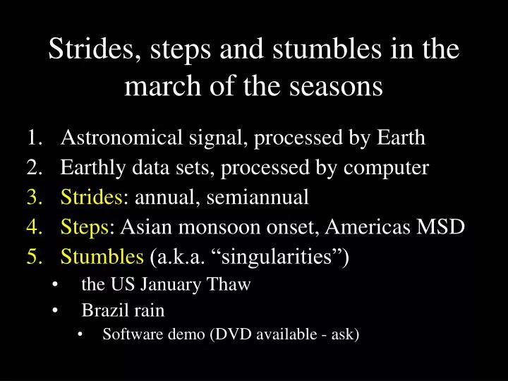
Strides, steps and stumbles in the march of the seasons. Astronomical signal, processed by Earth Earthly data sets, processed by computer Strides : annual, semiannual Steps : Asian monsoon onset, Americas MSD Stumbles (a.k.a. “singularities”) the US January Thaw Brazil rain

E N D
Strides, steps and stumbles in the march of the seasons • Astronomical signal, processed by Earth • Earthly data sets, processed by computer • Strides: annual, semiannual • Steps: Asian monsoon onset, Americas MSD • Stumbles (a.k.a. “singularities”) • the US January Thaw • Brazil rain • Software demo (DVD available - ask)
High frequency aspects of the mean seasonal cycle Brian Mapes University of Miami
Astronomical forcing(spherical Earth, circular orbit) equinox equinox solstice solstice
Temporal Fourier spectrum of annual insolation no forcing, just internal nonlinearitites sin(4pt/365d) Semiannual sin(2pt/365d) Annual
Annual cycle signal processing(by the Earth) Cloud, albedo heating Heat capacity temperature gravity pressure rotation web of feedbacks wind precip evaporation, advection humidity micro- physics vertical motion cloud
Annual cycle signal processing (by the computer) • Form mean daily climatologies: var (365 calendar days; lat, lon, level, dataset) • Compute mean, annual + semiannual harmonics mean, 2 amplitudes, 2 phases • Residual is called “HF” HF = climatology - annual - semiannual • Wavelet analysis of HF {dates, periods, amplitudes, significances of HF events}
Wavelet example • Paul wavelet • Sharp time localization • broad in frequency • Real part: max/min • Imaginary part: rise/fall • (Torrence and Compo 1998 BAMS)
Signal processed. Now what?? Fourier and wavelet coefficients form a supplement (index) to climatology. This doubles the size of the data set. ?? What to do with all this information ?? interactive GUI visualization tool
Outline of examples • Annual • “Easy” (local, thermal): Tsfc • Nonlocal: Z250 (jet streams) • Semiannual • Nonlinear: angular momentum and u250 • Statistical: 250mb eddy activity • Ter-annual and beyond • oceanic subtropical highs, monsoons
Simplest: annual harmonic of surface air T OBS GFDL CSM
Cold winter low tropospheric thickness?annual harmonic of Z250 OBS GFDL CSM
Local Hadley cells? Annual Harmonic of u at 200 hPa Jan 1 Apr 1 Annual Harmonic of atmos. heating
Outline of examples • Annual • “Easy” (local, thermal): Tsfc • Nonlocal: Z250 (jet streams) • Semiannual • Nonlinear: angular momentum and u250 • Statistical: 250mb eddy activity • Ter-annual and beyond • oceanic subtropical highs, monsoons
Semiannual harmonic of 250 hPa zonal wind(Weickmann & Chervin 1988) Jan min Jan max Apr Apr
Apr-Oct Jan Apr Apr-Oct Semiannual harmonic of 250 hPa zonal wind Jan Apr Apr OBS May+Nov HF total Apr Jun+Dec CSM
semiannual harmonic of 250 hPa zonal windsemiannual u in a forced/damped barotropic model forced with annual harmonic only of 200mb div (Huang & Sardeshmukh 2000) Apr-Oct Jan-Jul Apr-Oct total Apr-Oct Jan-Jul Apr-Oct A nonlinear overtone
Semiannual eddy (storm) activity Midwinter Suppression of Baroclinic Wave Activity in the Pacific Nakamura 1992 ABSTRACT Seasonal variations in baroclinic wave activity and jet stream structure in the Northern Hemisphere are investigated based upon over 20 years of daily data. Baroclinic wave activity at each grid point is represented for each day by an envelope function, the lowpass-filtered time series of the squared highpass-filtered geopotential height. Baroclinic wave activity over the Atlantic exhibits a single maximum in January, whereas in the Pacific it exhibits peaks in late autumn and in early spring and a significant weakening in midwinter, which is more evident at the tropopause level than near the surface. This suppression occurs despite the fact that the low-level baroclinity and the intensity of the jet stream are strongest in midwinter. Based on the analysis of 31-day running mean fields for individual winters, it is shown that over both the oceans baroclinic wave activity is positively correlated with the strength of the upper-tropospheric jet for wind speeds up to 45 m s 1. When the strength of the westerlies exceeds this optimal value, as it usually does over the western Pacific during midwinter, the correlation is negative: wave amplitude and the meridional fluxes of heat and zonal momentum all decrease with increasing wind speed. The phase speed of the waves increases with wind speed, while the steering level drops, which is indicative of the increasing effects of the mean flow advection and the trapping of the waves near the surface.
midwinter eddy minimumsemiannual amplitude (color) of a climatology of stdev of 9d sliding window v250Decently simulated by coupled model NCEP 1969-96 Oct+Apr maxima of eddy v variance CSM 1.3
Outline of examples • Annual • “Easy” (local, thermal): Tsfc • Nonlocal: Z250 (jet streams) • Semiannual • Nonlinear: angular momentum and u250 • Statistical: 250mb eddy activity • Ter-annual and beyond • oceanic subtropical highs, monsoons
Ter-annual variations of sea-level pressure HF total 10d 100d
CSM climate model HF total
Understanding SLP seasonality:Zonal mean total HF 10d 100d
Monsoon-related ~100d period high Oceanic (Aleutian) ~semiannual low Pacific ter-annual SLP schematic NH Winter High NH Summer Low
Outline of examples • Annual • “Easy” (local, thermal): Tsfc • Nonlocal: Z250 (jet streams) • Semiannual • Nonlinear: angular momentum and u250 • Statistical: 250mb eddy activity • Ter-annual and beyond • oceanic subtropical highs, monsoons
Linho and Wang 2002wavelet method EASM ISM WNPM EASM ISM WNPM
a model:decentISM onset, but poor at oceanic systems EASM ISM WNPM
North America at same time ENASM? EASM NAM ISM WNPM EASM ISM WNPM
June onset in southeast US(from CPC .25deg 1948-98 gauge data set)(mid-summer dip) Jun 1 Jul 1
5 Ter-annual midsummer structurehigh & dry in tropical Americas CMAP 23y mean obs. rain 1 dry July Aug NCEP 27 year (1969-96) SLP Gulf of Mexico area HF
Midsummer high in W. Atlantic 21 May- 10 June wet 3-27 July dry
Key features of Asian vs. American monsoons : a model experiment IPRC / ECHAM model: shown to have decent Asian onset, American midsummer drought Enhance monsoons by allowing each calendar day (solar declination) to last 5x24 hours. Summer continents get hotter, atm has time to equilibrate. (SST fixed to obs. for each calendar day)
April-Sept rainfall, exp-control:S. Asia wetter, Americas drier • S. Asia time series shows earlier (May) onset in exp • Stated regarding the control run, • Land-atm lags delay Asian monsoon onset behind its seasonal forcing by ~1mo. • Onset is the main disequilibrium of the Asian monsoon wrt seasonal forcing total May
April-Sept rainfall, exp-control:S. Asia wetter, Americas drier • Americas time series shows mid-summer drought earlier and drier in exp • Stated regarding the control run, • Land-atm lags prevent American midsummer drought from developing fully • Midsummer drought is the main disequilibrium of the American summer monsoon wrt seasonal forcing Jun July
Outline of examples • Ter-annual and beyond • oceanic subtropical highs • monsoons • Asian onset • American midsummer drought • These things are related
Chen, Hoerling and Dole 2001 Heating Eddy Z1000 w/o shear Eddy Z1000 July u(y,p)
Jul-Aug time slice time slice u300, zonal mean 60N Westerlies retreat to >30N in midsummer <0 Eq J F M A M J J A S O N D easterlies protrude to 30N suddenly in mid summer • WHY, in terms of [u] budget? • Not f[v]: ~barotropic; [v](t) wrong • [u’v’]: Tilted TUTTs, Tibetan High, Transients?
Winter Wiggles • Sub-ter-annual time scales: real ?? • ‘The January Thaw’ • a statistical phantom? (BAMS Jan 2001) • Brazilian rainfall
January Thaw lit. of 1919
missing this Boston, 1872-1965 Entire debate centers on this spike
Jan Revisit, withmore spatialaveraging • 1969-96 NCEP reanalysis surface air temperature • N. America mean • (think vdT/dy) 3K HF part unsmoothed daily T 5K Jun Jul 10d 100d
Winter Wiggles • Sub-ter-annual time scales: real ?? • ‘The January Thaw’ • a statistical phantom? (BAMS Jan 2001) • Brazilian rainfall
High High High High Where are those boxes? W. subtropical oceans
TAIWAN 25N May CMAP rainfall climatologies: CUBA 25N May SE BRAZIL 25S Nov. MADAGASCAR 25S Nov.
East Brazil rain gauge data ? Source: CPTEC Web site
SP & Rioclim. ? Source: Hotel inter-continental Web site