Download
1 / 56
570 likes | 1.03k Views
CIS 636 Introduction to Computer Graphics CG Basics 2 of 8: Rasterization and 2-D Clipping William H. Hsu Department of Computing and Information Sciences, KSU KSOL course pages: http://snipurl.com/1y5gc Course web site: http://www.kddresearch.org/Courses/CIS636

E N D
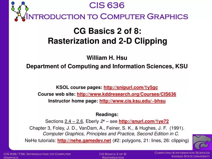
CIS 636Introduction to Computer Graphics CG Basics 2 of 8: Rasterization and 2-D Clipping William H. Hsu Department of Computing and Information Sciences, KSU KSOL course pages: http://snipurl.com/1y5gc Course web site: http://www.kddresearch.org/Courses/CIS636 Instructor home page: http://www.cis.ksu.edu/~bhsu Readings: Sections 2.4 – 2.6, Eberly 2e – see http://snurl.com/1ye72 Chapter 3, Foley, J. D., VanDam, A., Feiner, S. K., & Hughes, J. F. (1991). Computer Graphics, Principles and Practice, Second Edition in C. NeHe tutorials: http://nehe.gamedev.net(#2: polygons, 21: lines, 26: clipping) CIS 636/736: (Introduction to) Computer Graphics
Lecture Outline • Scan Conversion of Lines • Naïve algorithm • Midpoint algorithm (aka Bresenham’s) • Method of forward differences • Scan Conversion of Polygons • Scan line interpolation • Why it’s important: basis of shading/texturing, z-buffering • Scan Conversion of Circles and Ellipses • Aliasing and Antialiasing • Basic problem defined • Approaches CIS 636/736: (Introduction to) Computer Graphics
Online Recorded Lectures for CIS 636Introduction to Computer Graphics • Project Topics for CIS 636 • Computer Graphics Basics (8) • 1. Mathematical Foundations – Week 2 • 2. Rasterizing and 2-D Clipping – Week 3 • 3. OpenGL Primer 1 of 3 – Week 3 • 4. Detailed Introduction to 3-D Viewing – Week 4 • 5. OpenGL Primer 2 of 3 – Week 5 • 6. Polygon Rendering – Week 6 • 7. OpenGL Primer 3 of 3 – Week 8 • 8. Visible Surface Determination – Week 9 • Recommended Background Reading for CIS 636 • Shared Lectures with CIS 736 (Computer Graphics) • Regular in-class lectures (35) and labs (7) • Guidelines for paper reviews – Week 7 • Preparing term project presentations, demos for graphics – Week 11 CIS 636/736: (Introduction to) Computer Graphics
Scan Converting Lines Line Drawing • Draw a line on a raster screen between two points • What’s wrong with the statement of the problem? • it doesn’t say anything about which points are allowed as endpoints • it doesn’t give a clear meaning to “draw” • it doesn’t say what constitutes a “line” in the raster world • it doesn’t say how to measure the success of a proposed algorithm Problem Statement • Given two points P and Q in the plane, both with integer coordinates, determine which pixels on a raster screen should be on in order to make a picture of a unit-width line segment starting at P and ending at Q Adapted from slides © 2005 A. VanDam, Brown University. Reused with permission. CIS 636/736: (Introduction to) Computer Graphics
Finding the next pixel Special case: • Horizontal Line: Draw pixel P and increment the x coordinate value by one to get the next pixel. • Vertical Line: Draw pixel P and increment the y coordinate value by one to get the next pixel. • Perfect Diagonal Line: Draw pixel P and increment both the x and the y coordinate by one to get the next pixel. • What should we do in the general case? • Increment the x coordinate by 1 and choose the point closest to the line. • But how do we measure “closest”? Adapted from slides © 2005 A. VanDam, Brown University. Reused with permission. CIS 636/736: (Introduction to) Computer Graphics
Vertical Distance • Why can we use the vertical distance as a measure of which point is closer? • because the vertical distance is proportional to the actual distance • how do we show this? • with congruent triangles • By similar triangles we can see that the true distances to the line (in blue) are directly proportional to the vertical distances to the line (in black) for each point • Therefore, the point with the smaller vertical distance to the line is the closest to the line (x1, y1) (x2, y2) Adapted from slides © 2005 A. VanDam, Brown University. Reused with permission. CIS 636/736: (Introduction to) Computer Graphics
Strategy 1: IncrementalAlgorithm [1] The Basic Algorithm • Find the equation of the line that connects the two points P and Q • Starting with the leftmost point P, increment xi by 1 to calculate yi= mxi+ B where m = slope, B = y intercept • Intensify the pixel at (xi, Round(yi)) where Round (yi) = Floor (0.5 + yi) The Incremental Algorithm: • Each iteration requires a floating-point multiplication • therefore, modify the algorithm. • yi+1= mxi+1+ B = m(xi+x)+ B = yi + m x • If x = 1, then yi+1 = yi+ m • At each step, we make incremental calculations based on the preceding step to find the next y value Adapted from slides © 2005 A. VanDam, Brown University. Reused with permission. CIS 636/736: (Introduction to) Computer Graphics
Strategy 1: IncrementalAlgorithm [2] Adapted from slides © 2005 A. VanDam, Brown University. Reused with permission. CIS 636/736: (Introduction to) Computer Graphics
Example Code // Incremental Line Algorithm // Assumes –1 <= m <= 1, x0 < x1 void Line(int x0, int y0, int x1, int y1, int value) { int x; float y; float dy = y1 – y0; float dx = x1 – x0; float m = dy / dx; y = y0; for (x = x0; x < x1; x++) { WritePixel(x, Round(y), value); y = y + m; } } Adapted from slides © 2005 A. VanDam, Brown University. Reused with permission. CIS 636/736: (Introduction to) Computer Graphics
Problems with IncrementalAlgorithm void Line(int x0, int y0, int x1, int y1, int value) { int x; float y; float dy = y1 – y0; float dx = x1 – x0; float m = dy / dx; y = y0; for (x = x0; x < x1; x++) { WritePixel(x, Round(y), value); y = y + m; } } Rounding takes time Since slope is fractional, need special case for vertical lines Adapted from slides © 2005 A. VanDam, Brown University. Reused with permission. CIS 636/736: (Introduction to) Computer Graphics
Strategy 2: Midpoint Line Algorithm [1] • Assume line’s slope is shallow and positive (0 < slope < 1); other slopes can be handled by suitable reflections about principal axes • Call lower left endpoint (x0, y0) and upper right endpoint (x1, y1) • Assume we have just selected pixel P at (xp, yp) • Next, must choose between • pixel to right (E pixel) • one right and one up (NE pixel) • Let Q be intersection point of line being scan-converted with grid line x = xp +1 Adapted from slides © 2005 A. VanDam, Brown University. Reused with permission. CIS 636/736: (Introduction to) Computer Graphics
Strategy 2: Midpoint Line Algorithm [2] NE pixel Q Midpoint M E pixel Previous pixel Choices for current pixel Choices for next pixel Adapted from slides © 2005 A. VanDam, Brown University. Reused with permission. CIS 636/736: (Introduction to) Computer Graphics
Strategy 2: Midpoint Line Algorithm [3] • The line passes between E and NE • The point that is closer to the intersection point Q must be chosen • Observe on which side of the line the midpoint M lies: • E is closer to the line if the midpoint M lies above the line, i.e., the line crosses the bottom half • NE is closer to the line if the midpoint M lies below the line, i.e., the line crosses the top half • The error, the vertical distance between the chosen pixel and the actual line, is always ≤ ½ • The algorithm chooses NE as the next pixel for the line shown • Now, find a way to calculate on which side of the line the midpoint lies Adapted from slides © 2005 A. VanDam, Brown University. Reused with permission. CIS 636/736: (Introduction to) Computer Graphics
The Line Line equation as a function f(x): • y = f(x) = m*x + B = dy/dx*x + B Line equation as an implicit function: • F(x, y)= a*x + b*y + c = 0 for coefficients a, b, c, where a, b ≠ 0 from above, y*dx = dy*x + B*dx so a = dy, b = -dx, c = B*dx, a >0 for y0< y1 Properties (proof by case analysis): • F(xm, ym) = 0 when any point M is on the line • F(xm, ym) < 0 when any point M is above the line • F(xm, ym) > 0 when any point M is below the line • Our decision will be based on the value of the function at the midpoint M at (xp + 1, yp + ½) Adapted from slides © 2005 A. VanDam, Brown University. Reused with permission. CIS 636/736: (Introduction to) Computer Graphics
Decision Variable Decision Variable d: • We only need the sign of F(xp+ 1, yp + ½) to see where the line lies, and then pick the nearest pixel • d = F(xp + 1, yp + ½) - if d > 0 choose pixel NE - if d < 0 choose pixel E - if d = 0 choose either one consistently How do we incrementally update d? • On the basis of picking E or NE, figure out the location of M for the next grid line, and the corresponding value of d = F(M) for that grid line Adapted from slides © 2005 A. VanDam, Brown University. Reused with permission. CIS 636/736: (Introduction to) Computer Graphics
E Pixel Chosen M is incremented by one step in the x direction dnew = F(xp + 2, yp + ½) = a(xp + 2) + b(yp + ½) + c dold = a(xp + 1)+ b(yp + ½)+ c • Subtract dold from dnew to get the incremental difference E dnew= dold+ a E= a = dy • Gives value of decision variable at next step incrementally without computing F(M) directly dnew= dold + E= dold+ dy • E can be thought of as the correction or update factor to take dold to dnew • It is referred to as the forward difference Adapted from slides © 2005 A. VanDam, Brown University. Reused with permission. CIS 636/736: (Introduction to) Computer Graphics
NE Pixel Chosen M is incremented by one step each in both the x and y directions dnew= F(xp + 2, yp + 3/2) = a(xp + 2)+ b(yp + 3/2)+ c • Subtract dold from dnew to get the incremental difference dnew = dold + a + b NE = a + b = dy – dx • Thus, incrementally, dnew = dold + NE = dold + dy – dx Adapted from slides © 2005 A. VanDam, Brown University. Reused with permission. CIS 636/736: (Introduction to) Computer Graphics
Summary [1] • At each step, the algorithm chooses between 2 pixels based on the sign of the decision variable calculated in the previous iteration. • It then updates the decision variable by adding either E or NE to the old value depending on the choice of pixel. Simple additions only! • First pixel is the first endpoint (x0, y0), so we can directly calculate the initial value of d for choosing between E and NE. Adapted from slides © 2005 A. VanDam, Brown University. Reused with permission. CIS 636/736: (Introduction to) Computer Graphics
Summary [2] • First midpoint for first d = dstartis at (x0 + 1, y0 + ½) • F(x0 + 1, y0 + ½) = a(x0 + 1) + b(y0 + ½) + c = a * x0 + b * y0 + c + a + b/2 = F(x0, y0) + a + b/2 • But (x0, y0) is point on the line and F(x0, y0) = 0 • Therefore, dstart = a + b/2 = dy – dx/2 • use dstart to choose the second pixel, etc. • To eliminate fraction in dstart : • redefine F by multiplying it by 2; F(x,y) = 2(ax + by + c) • this multiplies each constant and the decision variable by 2, but does not change the sign • Bresenham’s line algorithm: same but doesn’t generalize as nicely to circles and ellipses Adapted from slides © 2005 A. VanDam, Brown University. Reused with permission. CIS 636/736: (Introduction to) Computer Graphics
Example Code void MidpointLine(int x0, int y0, int x1, int y1, int value) { int dx = x1 - x0; int dy = y1 - y0; int d = 2 * dy - dx; int incrE = 2 * dy; int incrNE = 2 * (dy - dx); int x = x0; int y = y0; writePixel(x, y, value); while (x < x1) { if (d <= 0) { //East Case d = d + incrE; } else { // Northeast Case d = d + incrNE; y++; } x++; writePixel(x, y, value); } /* while */ } /* MidpointLine */ Adapted from slides © 2005 A. VanDam, Brown University. Reused with permission. CIS 636/736: (Introduction to) Computer Graphics
Generic Polygons Adapted from slides © 2005 A. VanDam, Brown University. Reused with permission. CIS 636/736: (Introduction to) Computer Graphics
© 2007 Disney/Pixar © 2001 – 2007 DreamWorks Animation SKG © 2006 Warner Brothers ~ Intermission ~ Take A Break! CIS 636/736: (Introduction to) Computer Graphics
N 2 Polygon Mesh Shading [1] • Illumination intensity interpolation • Gouraud shading • use for polygon approximations to curved surfaces • Linearly interpolate intensity along scan lines • eliminates intensity discontinuities at polygon edges; still have gradient discontinuities, mach banding is improved, not eliminated • must differentiate desired creases from tesselation artifacts (edges of a cube vs. edges on tesselated sphere) • Step 1: calculate bogus vertex normals as average of surrounding polygons’ normals: • neighboring polygons sharing vertices and edges approximate smoothly curved surfaces and won’t have greatly differing surface normals; therefore this approximation is reasonable N 1 N More generally: v n = 3 or 4 usually N 4 N 3 Adapted from slides © 2005 A. VanDam, Brown University. Reused with permission. CIS 636/736: (Introduction to) Computer Graphics
Polygon Mesh Shading [2] • Illumination intensity interpolation (cont.) • Step 2: interpolate intensity along polygon edges • Step 3: interpolate along scan lines scan line Adapted from slides © 2005 A. VanDam, Brown University. Reused with permission. CIS 636/736: (Introduction to) Computer Graphics
(0, 17) (0, 17) (17, 0) (17, 0) Scan Converting Circles [1] Version 1: really bad For x = – R to R y = sqrt(R •R – x •x); Pixel (round(x), round(y)); Pixel (round(x), round(-y)); Version 2: slightly less bad For x = 0 to 360 Pixel (round (R • cos(x)), round(R • sin(x))); Adapted from slides © 2005 A. VanDam, Brown University. Reused with permission. CIS 636/736: (Introduction to) Computer Graphics
(0, 17) (17, 0) Scan Converting Circles [2] Version 3: better! • Midpoint Circle Algorithm: • First octant generated by algorithm • Other octants generated by symmetry First octant Second octant Adapted from slides © 2005 A. VanDam, Brown University. Reused with permission. CIS 636/736: (Introduction to) Computer Graphics
(x0 + a, y0 + b) R (x0, y0) (x-x0)2 + (y-y0)2 = R2 Midpoint Circle Algorithm • Symmetry: If (x0 + a, y0 + b) is on the circle, so are (x0± a, y0± b) and (x0± b, y0± a); hence there’s an 8-way symmetry. • BUT, keep in mind that there are always issues when rounding points on a circle to integers Adapted from slides © 2005 A. VanDam, Brown University. Reused with permission. CIS 636/736: (Introduction to) Computer Graphics
(x0, y0) Using the Symmetry • We will scan top right 1/8 of circle of radius R • It starts at (x0, y0 + R) • Let’s use another incremental algorithm with a decision variable evaluated at midpoint Adapted from slides © 2005 A. VanDam, Brown University. Reused with permission. CIS 636/736: (Introduction to) Computer Graphics
Sketch of Incremental Algorithm E y = y0 + R; x = x0; Pixel(x, y); For (x = x0+1; (x – x0) > (y – y0); x++) { if (decision_var < 0) { /* move east */ update decision_var; } else { /* move south east */ update decision_var; y--; } Pixel(x, y); } • (decision_var will be defined momentarily) • Note: can replace all occurrences of x0 and y0 with 0, 0, Pixel (x0 + x, y0 + y) with Pixel (x, y) • Essentially a shift of coordinates SE Adapted from slides © 2005 A. VanDam, Brown University. Reused with permission. CIS 636/736: (Introduction to) Computer Graphics
What We Need for Incremental Algorithm • Need a decision variable, i.e., something that is negative if we should move E, positive if we should move SE (or vice versa). • Follow line strategy: Use the implicit equation of circle F(x,y) = x2 + y2 – R2 = 0 F(x,y) is zero on the circle, negative inside it, positive outside • If we are at pixel (x, y), examine (x + 1, y) and (x + 1, y – 1) • Again compute F at the midpoint = F(midpoint) Adapted from slides © 2005 A. VanDam, Brown University. Reused with permission. CIS 636/736: (Introduction to) Computer Graphics
M ME SE MSE æ ö 1 + - ç ÷ x 1 , y 2 è ø 2 æ ö æ ö 1 1 + - = + + - - 2 2 ç ÷ ç ÷ F x 1 , y ( x 1 ) y R è 2 ø è 2 ø Decision Variable • Evaluate F(x,y) = x2 + y2 – R2 at the point • What we are asking is this: “Is positive or negative?” • If it is negative there, this midpoint is inside the circle, so the vertical distance to the circle is less at (x + 1, y) than at (x + 1, y–1). • If it is positive, the opposite is true. P = (xp, yp) Adapted from slides © 2005 A. VanDam, Brown University. Reused with permission. CIS 636/736: (Introduction to) Computer Graphics
+ = + + - 2 2 d (( x 1 , y ), Circ ) ( x 1 ) y R + - = + + - - 2 2 d (( x 1 , y 1 ), Circ ) ( x 1 ) ( y 1 ) R + + + + - 2 2 2 2 ( x 1 ) y or ( x 1 ) ( y 1 ) Is this the right decision variable? • It makes our decision based on vertical distance • For lines, that was ok , since d and dvertwere proportional • For circles, no longer true: • We ask which d is closer to zero, i.e., which of the two values below is closer to R: Adapted from slides © 2005 A. VanDam, Brown University. Reused with permission. CIS 636/736: (Introduction to) Computer Graphics
+ + - + + - = - 2 2 2 2 [( x 1 ) y ] [( x 1 ) ( y 1 ) ] 2 y 1 Alternate Specification [1] • We could ask instead (*) “Is (x + 1)2 + y2 or (x + 1)2 + (y – 1)2 closer to R2?” • The two values in equation (*) above differ by (0, 17) (1, 17) E FE = 12 + 172 = 290 (1, 16) FSE = 12 + 162 = 257 SE FE – FSE = 290 – 257 = 33 2y – 1 = 2(17) – 1 = 33 Adapted from slides © 2005 A. VanDam, Brown University. Reused with permission. CIS 636/736: (Introduction to) Computer Graphics
æ ö 1 - ç ÷ ( 2 y 1 ) è 2 ø - + + - 2 2 2 R [( x 1 ) ( y 1 ) ] 1 - y ( 2 1 ) < 2 1 2 2 2 < - + + + - - 0 y ( x 1 ) ( y 1 ) R 2 1 2 2 2 < + + - + + - - 0 ( x 1 ) y 2 y 1 y R 2 1 < + 2 + 2 - + - 2 0 ( x 1 ) y y R 2 2 æ ö 1 1 < + + - + - 2 2 ç ÷ 0 ( x 1 ) y R è 2 ø 4 Alternate Specification [2] • So the second value, which is always the lesser, is closer if its difference from R2 is less than i.e., if then so so so Adapted from slides © 2005 A. VanDam, Brown University. Reused with permission. CIS 636/736: (Introduction to) Computer Graphics
2 æ ö 1 1 = + + - + - 2 2 ç ÷ d 1 ( x 1 ) y R 2 4 è ø 2 æ ö 1 = + + - - 2 2 ç ÷ d 2 ( x 1 ) y R 2 è ø Alternate Specification [3] • So the radial distance decision is whether is positive or negative • And the vertical distance decision is whether is positive or negative; d1 and d2 are apart. • The integer d1 is positive only if d2 + is positive (except special case where d2 = 0). • Hence, aside from ambiguous cases, the two are the same. Adapted from slides © 2005 A. VanDam, Brown University. Reused with permission. CIS 636/736: (Introduction to) Computer Graphics
2 æ ö 1 + + - = - 2 2 ç ÷ F ( x , y ) ( x 1 ) y R 2 ø è + - ( x 1 , y ) F ( x , y ) F D = + ( x , y ) 2 x 3 E + - - F x y F x y ( 1 , 1 ) ( , ) D = + - + ( x , y ) 2 x 3 2 y 2 SE Incremental Computation, Again [1] • How should we compute the value of at successive points? • Answer: Note that is just and that is just Adapted from slides © 2005 A. VanDam, Brown University. Reused with permission. CIS 636/736: (Introduction to) Computer Graphics
F F’ F’’ Incremental Computation, Again [2] • So if we move E, update by adding 2x + 3 • And if we move SE, update by adding 2x + 3 – 2y + 2. • Note that the forward differences of a 1st degree polynomial were constants and those of a 2nd degree polynomial are 1st degree polynomials; this “first order forward difference,” like a partial derivative, is one degree lower. Let’s make use of this property. Adapted from slides © 2005 A. VanDam, Brown University. Reused with permission. CIS 636/736: (Introduction to) Computer Graphics
D = + 3 ( x , y ) 2 x E D + - D = ( x 1 , y ) ( x , y ) 2 E E D + - - D = ( x 1 , y 1 ) ( x , y ) 2 E E D + - D = ( x 1 , y ) ( x , y ) 2 SE SE D + - - D = ( x 1 , y 1 ) ( x , y ) 4 SE SE Second Differences [1] • The function is linear, and hence amenable to incremental computation, viz: • Similarly Adapted from slides © 2005 A. VanDam, Brown University. Reused with permission. CIS 636/736: (Introduction to) Computer Graphics
Second Differences [2] • So for any step, we can compute new ΔE(x, y) from old ΔE(x, y) by adding an appropriate second constant increment – we update the update terms as we move. • This is also true of ΔSE(x, y) • Having previously drawn pixel (a,b), in current iteration, we decide between drawing pixel at (a + 1, b) and (a + 1, b – 1), using previously computed d(a, b). • Having drawn the pixel, we must update d(a, b) for use next time; we’ll need to find either d(a + 1, b) or d(a + 1, b – 1) depending on which pixel we chose. • Will require adding ΔE(a, b)or ΔSE(a, b) to d(a, b) • So we… • Look at d(i) to decide which to draw next, update x and y • Update d using ΔE(a,b) or ΔSE(a,b) • Update each of ΔE(a,b) and ΔSE(a,b) for future use • Draw pixel Adapted from slides © 2005 A. VanDam, Brown University. Reused with permission. CIS 636/736: (Introduction to) Computer Graphics
Midpoint Eighth-Circle Algorithm MEC (R) /* 1/8th of a circle w/ radius R */ { int x = 0, y = R; int delta_E, delta_SE; float decision; delta_E = 2*x + 3; delta_SE = 2(x-y) + 5; decision = (x+1)*(x+1) + (y + 0.5)*(y + 0.5) –R*R; Pixel(x, y); while( y > x ) { if (decision > 0) {/* Move east */ decision += delta_E; delta_E += 2; delta_SE += 2; } else {/* Move SE */ y--; decision += delta_SE; delta_E += 2; delta_SE += 4; } x++; Pixel(x, y); } } Adapted from slides © 2005 A. VanDam, Brown University. Reused with permission. CIS 636/736: (Introduction to) Computer Graphics
Analysis • Uses a float! • 1 test, 3 or 4 additions per pixel • Initialization can be improved • Multiply everything by 4 No Floats! • This makes the components even, but the sign of the decision variable remains the same Questions • Are we getting all pixels whose distance from the circle is less than ½? • Why is “x < y” the right stopping criterion? • What if it were an ellipse? Adapted from slides © 2005 A. VanDam, Brown University. Reused with permission. CIS 636/736: (Introduction to) Computer Graphics
Other Scan Conversion Problems • Patterned primitives • Aligned Ellipses • Non-integer primitives • General conics Adapted from slides © 2005 A. VanDam, Brown University. Reused with permission. CIS 636/736: (Introduction to) Computer Graphics
Patterned Lines • Patterned line from P to Q is not same as patterned line from Q to P. • Patterns can be geometric or cosmetic • Cosmetic: Texture applied after transformations • Geometric: Pattern subject to transformations Cosmetic patterned line Geometric patterned line P Q P Q Adapted from slides © 2005 A. VanDam, Brown University. Reused with permission. CIS 636/736: (Introduction to) Computer Graphics
Geometric vs. Cosmetic Pattern + Adapted from slides © 2005 A. VanDam, Brown University. Reused with permission. CIS 636/736: (Introduction to) Computer Graphics
2 2 x y + = 1 2 2 a b + = 2 2 2 2 2 2 b x a y a b D D SE E Aligned Ellipses • Equation is i.e, • Computation of and is similar • Only 4-fold symmetry • When do we stop stepping horizontally and switch to vertical? Adapted from slides © 2005 A. VanDam, Brown University. Reused with permission. CIS 636/736: (Introduction to) Computer Graphics
Ñ é ù ¶ ¶ F F ( x , y ), ( x , y ) ê ú ¶ ¶ x y ë û ¶ ¶ F F - > ( x , y ) ( x , y ) 0 ¶ ¶ x y Direction-Changing Criterion [1] • When the absolute value of the slope of the ellipse is more than 1, viz: • How do you check this? At a point (x,y) for which F(x,y) = 0, a vector perpendicular to the level set is F(x,y) which is • This vector points more right than up when Adapted from slides © 2005 A. VanDam, Brown University. Reused with permission. CIS 636/736: (Introduction to) Computer Graphics
¶ F = 2 ( x , y ) 2 a x ¶ x ¶ F = 2 ( x , y ) 2 b y ¶ y - > 2 2 2 a x 2 b y 0 - > 2 2 a x b y 0 Direction-Changing Criterion [2] • In our case, and so we check for i.e. • This, too, can be computed incrementally Adapted from slides © 2005 A. VanDam, Brown University. Reused with permission. CIS 636/736: (Introduction to) Computer Graphics
Problems with Aligned Ellipses • Now in ENE octant, not ESE octant • This problem is due to aliasing – much more on this later Adapted from slides © 2005 A. VanDam, Brown University. Reused with permission. CIS 636/736: (Introduction to) Computer Graphics
http://snurl.com/1yw63 http://snurl.com/1yw67 http://snurl.com/1yw5z Unweighted (box) Weighted (cone) Aliasing and Antialiasing • Definition • Effect causing two continuous signals to become indistinguishable (aliases) • Occurs when sampled • Signals: actual mathematical object (line, polygon, ellipse) • General examples: distortion, artifacts • Specific Examples of Aliasing • Spatial aliasing: Moiré pattern (aka Moiré vibration) • Jaggies in line, polygon, ellipse scan conversion • Temporal aliasing in animation (later) • Antialiasing: Techniques for Prevention • (Unweighted) area sampling • Pixel weighting: weighted area sampling CIS 636/736: (Introduction to) Computer Graphics
Non-Integer Primitives and General Conics • Non-Integer Primitives • Initialization is harder • Endpoints are hard, too • making Line (P,Q) and Line (Q,R) join properly is a good test • Symmetry is lost • General Conics • Very hard--the octant-changing test is tougher, the difference computations are tougher, etc. • do it only if you have to. • Note that when we get to drawing gray-scale conics, we will find that this task is easier than drawing B/W conics; if we had solved this problem first, life would have been easier. Adapted from slides © 2005 A. VanDam, Brown University. Reused with permission. CIS 636/736: (Introduction to) Computer Graphics