Download
1 / 46
460 likes | 851 Views
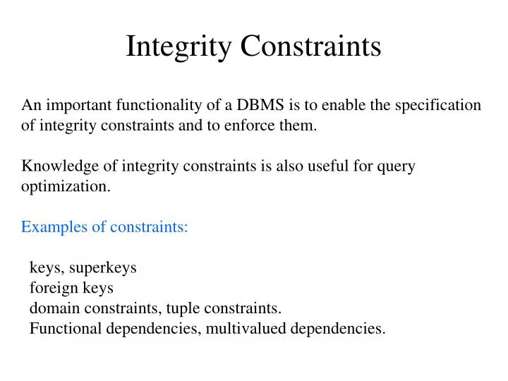
Integrity Constraints. An important functionality of a DBMS is to enable the specification of integrity constraints and to enforce them. Knowledge of integrity constraints is also useful for query optimization. Examples of constraints: keys, superkeys foreign keys

E N D
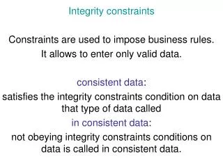
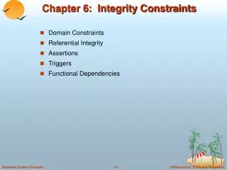
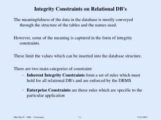
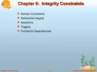
Integrity Constraints An important functionality of a DBMS is to enable the specification of integrity constraints and to enforce them. Knowledge of integrity constraints is also useful for query optimization. Examples of constraints: keys, superkeys foreign keys domain constraints, tuple constraints. Functional dependencies, multivalued dependencies.
Keys A minimal set of attributes that uniquely identifies the tuple (I.e., there is no pair of tuples with the same values for the key attributes): Person: social security number name name + address name + address + age Perfect keys are often hard to find, but organizations usually invent something anyway. Superkey: a set of attributes that contains a key. A relation may have multiple keys:(but only one primary key) employee number, social-security number
Foreign Key Constraints Product: name manufacturer description gizmo G-sym great stuff E-gizmo G-sym even better Purchase: buyer price product Joe $20 gizmo Jack $20 E-gizmo An attribute of a relation R is must refer to a key of a relation S. (need to be careful during deletions).
Functional Dependencies Definition: Two tuples that agree on the attributes A1,…,An must also agree on the attributes B1,…, Bm Formally: A , A , … A B , B , … B 1 2 m 1 2 n If A1,…,An is a key, then A1,…,An Attributes(R) - A1,…,An
Example Problem in Designing Schema Name SSN Phone Number Fred 123-321-99 (201) 555-1234 Fred 123-321-99 (206) 572-4312 Joe 909-438-44 (908) 464-0028 Joe 909-438-44 (212) 555-4000 Problems: - redundancy - update anomalies - deletion anomalies
Relation Decomposition Break the relation into two relations: Name SSN Fred 123-321-99 Joe 909-438-44 Name Phone Number Fred (201) 555-1234 Fred (206) 572-4312 Joe (908) 464-0028 Joe (212) 555-4000
Boyce-Codd Normal Form A simple condition for removing anomalies from relations: A relation R is in BCNF if and only if: Whenever there is a nontrivial dependency for R , it is the case that { } is a super-key for R. A , A , … A B 1 2 n A , A , … A 1 2 n In English (though a bit vague): Whenever a set of attributes of R is determining another attribute, should determine all the attributes of R.
Querying Relational Databases • Relational algebra: an operational language • Relational calculus: a declarative language • tuple relational calculus (TRC) • domain relational calculus (DRC) • Codd: • The two are equivalent (sort of) • They provide a yardstick for other languages (concept of relational completeness) • SQL: influenced mostly by TRC • Query execution plans: relational algebra
Relational Algebra • Expresses functions from sets to a set. • Basic Set Operators • union, intersection, difference, but no complement. (watch for comparable sets) • Selection • Projection • Cartesian Product • Joins (equi-join, natural join, semi-join)
Set Operations • Binary operations • Result is table(set) with same attributes • Sets must be compatible! • R1(A1,A2,A3), R2(B1,B2,B3) • Domain(Ai)=Domain(Bi) • Union: all tuples in R1 or R2 • Intersection: all tuples in R1 and R2 • Difference: all tuples in R1 and not in R2 • No complement… what’s the universe?
Selection • Output a subset of the tuples in a relation which satisfy a given condition • Unary operation… returns set with same attributes, but ‘selects’ rows • Use and, or, not, >, <… to build condition
Projection • Unary operation, selects columns • Returned schema is different, so returned tuples are not subset of original set, like they are in selection • Eliminates duplicate tuples
Cartesian Product • Binary Operation • Result is tuples combining any element of R1 with any element of R2, for R1xR2 • Schema is union of Schema(R1) & Schema(R2). • Doesn’t happen much in practice (in fact, we try to avoid it).
Join • Most often used… • Combines two relations, selecting only related tuples • Equivalent to a cross product followed by selection and projection • Resulting schema has all attributes of the two relations, but one copy of join condition attributes.
Exercises Product ( name, price, category, maker) Purchase (buyer, seller, store, product) Company (cname, stock price, country) Person( pname, phone number, city) Ex #1: Find people who bought telephony products. Ex #2: Find names of people who bought American products Ex #3: Find names of people who bought American products and did not buy French products Ex #4: Find names of people who bought American products and they live in Seattle. Ex #5: Find people who bought stuff from Joe or bought products from a company whose stock prices is more than $50.
Tuple Relational Calculus • Find products costing at least $500 in the shoes category: • {T | T in Product & T.Price > 500 & T.Category=“Shoes”}
SQL Introduction Standard language for querying and manipulating data Structured Query Language Many standards out there: SQL92, SQL2, SQL3. Vendors support various subsets of these, but all of what we’ll be talking about. Basic form: (many many more bells and whistles in addition) Select attributes From relations (possibly multiple, joined) Where conditions (selections)
SQL Outline • select-project-join • attribute referencing, select distinct • nested queries • grouping and aggregation • updates • laundry list
Selections SELECT * FROM Company WHERE country=‘USA’ AND stockPrice > 50 You can use: attribute names of the relation(s) used in the FROM. comparison operators: =, <>, <, >, <=, >= apply arithmetic operations: stockprice*2 operations on strings (e.g., “||” for concatenation). Lexicographic order on strings. Pattern matching: s LIKE p Special stuff for comparing dates and times.
Projections and Ordering Results Select only a subset of the attributes SELECT name, stock price FROM Company WHERE country=‘USA’ AND stockPrice > 50 Rename the attributes in the resulting table SELECT name AS company, stockprice AS price FROM Company WHERE country=‘USA’ AND stockPrice > 50 ORDER BY country, name
Joins SELECT name, store FROM Person, Purchase WHERE name=buyer AND city=‘Seattle’ AND product=‘gizmo’ Product ( name, price, category, maker) Purchase (buyer, seller, store, product) Company (name, stock price, country) Person( name, phone number, city)
Disambiguating Attributes Find names of people buying telephony products: SELECT Person.name FROM Person, Purchase, Product WHERE Person.name=buyer AND product=Product.name AND Product.category=‘telephony’ Product ( name, price, category, maker) Purchase (buyer, seller, store, product) Person( name, phone number, city)
Tuple Variables Find pairs of companies making products in the same category SELECT product1.maker, product2.maker FROM Product AS product1, Product AS product2 WHERE product1.category=product2.category AND product1.maker <> product2.maker Product ( name, price, category, maker)
First Unintuitive SQLism SELECT R.A FROM R,S,T WHERE R.A=S.A OR R.A=T.A Looking for R I (S U T) But what happens if T is empty?
Union, Intersection, Difference (SELECT name FROM Person WHERE City=‘Seattle’) UNION (SELECT name FROM Person, Purchase WHERE buyer=name AND store=‘The Bon’) Similarly, you can use INTERSECT and EXCEPT. You must have the same attribute names (otherwise: rename).
Subqueries SELECT Purchase.product FROM Purchase WHERE buyer = (SELECT name FROM Person WHERE social-security-number = ‘123 - 45 - 6789’); In this case, the subquery returns one value. If it returns more, it’s a run-time error.
Subqueries Returning Relations Find companies who manufacture products bought by Joe Blow. SELECT Company.name FROM Company, Product WHERE Company.name=maker AND Product.name IN (SELECT product FROM Purchase WHERE buyer = ‘Joe Blow’); You can also use: s > ALL R s > ANY R EXISTS R
Correlated Queries Find movies whose title appears more than once. SELECT title FROM Movie AS Old WHERE year < ANY (SELECT year FROM Movie WHERE title = Old.title); Movie (title, year, director, length) Movie titles are not unique (titles may reappear in a later year). Note scope of variables
Removing Duplicates SELECTDISTINCT Company.name FROM Company, Product WHERE Company.name=maker AND (Product.name,price) IN (SELECT product, price) FROM Purchase WHERE buyer = ‘Joe Blow’);
Conserving Duplicates The UNION, INTERSECTION and EXCEPT operators operate as sets, not bags. (SELECT name FROM Person WHERE City=‘Seattle’) UNION ALL (SELECT name FROM Person, Purchase WHERE buyer=name AND store=‘The Bon’)
Aggregation SELECT Sum(price) FROM Product WHERE manufacturer=‘Toyota’ SQL supports several aggregation operations: SUM, MIN, MAX, AVG, COUNT Except COUNT, all aggregations apply to a single attribute SELECT Count(*) FROM Purchase
Grouping and Aggregation Usually, we want aggregations on certain parts of the relation. Find how much we sold of every product SELECT product, Sum(price) FROM Product, Purchase WHERE Product.name = Purchase.product GROUP BY Product.name 1. Compute the relation (I.e., the FROM and WHERE). 2. Group by the attributes in the GROUP BY 3. Select one tuple for every group (and apply aggregation) SELECT can have (1) grouped attributes or (2) aggregates.
HAVING Clause Same query, except that we consider only products that had at least 100 buyers. SELECT product, Sum(price) FROM Product, Purchase WHERE Product.name = Purchase.product GROUP BY Product.name HAVING Count(buyer) > 100 HAVING clause contains conditions on aggregates.
Modifying the Database We have 3 kinds of modifications: insertion, deletion, update. Insertion: general form -- INSERT INTO R(A1,…., An) VALUES (v1,…., vn) Insert a new purchase to the database: INSERT INTO Purchase(buyer, seller, product, store) VALUES (‘Joe’, ‘Fred’, ‘wakeup-clock-espresso-machine’ ‘The Sharper Image’) If we don’t provide all the attributes of R, they will be filled with NULL. We can drop the attribute names if we’re providing all of them in order.
Data Definition in SQL • So far, SQL operations on the data. • Data definition: defining the schema. • Create tables • Delete tables • Modify table schema • But first: • Define data types. • Finally: define indexes.
Data Types in SQL • Character strings (fixed of varying length) • Bit strings (fixed or varying length) • Integer (SHORTINT) • Floating point • Dates and times • Domains will be used in table declarations. • To reuse domains: • CREATE DOMAIN address AS VARCHAR(55)
Creating Tables CREATE TABLE Person( name VARCHAR(30), social-security-number INTEGER, age SHORTINT, city VARCHAR(30), gender BIT(1), Birthdate DATE );
Creating Indexes CREATE INDEX ssnIndex ON Person(social-security-number) Indexes can be created on more than one attribute: CREATE INDEX doubleindex ON Person (name, social-security-number) Why not create indexes on everything?
Defining Views Views are relations, except that they are not physically stored. They are used mostly in order to simplify complex queries and to define conceptually different views of the database to different classes of users. View: purchases of telephony products: CREATE VIEW telephony-purchases AS SELECT product, buyer, seller, store FROM Purchase, Product WHERE Purchase.product = Product.name AND Product.category = ‘telephony’
A Different View CREATE VIEW Seattle-view AS SELECT buyer, seller, product, store FROM Person, Purchase WHERE Person.city = ‘Seattle’ AND Person.name = Purchase.buyer We can later use the views: SELECT name, store FROM Seattle-view, Product WHERE Seattle-view.product = Product.name AND Product.category = ‘shoes’ What’s really happening when we query a view??
Updating Views How can I insert a tuple into a table that doesn’t exist? CREATE VIEW bon-purchase AS SELECT store, seller, product FROM Purchase WHERE store = ‘The Bon Marche’ If we make the following insertion: INSERT INTO bon-purchase VALUES (‘the Bon Marche’, ‘Joe’, ‘Denby Mug’) We can simply add a tuple (‘the Bon Marche’, ‘Joe’, NULL, ‘Denby Mug’) to relation Purchase.
Non-Updatable Views CREATE VIEW Seattle-view AS SELECT seller, product, store FROM Person, Purchase WHERE Person.city = ‘Seattle’ AND Person.name = Purchase.buyer How can we add the following tuple to the view? (‘Joe’, ‘Shoe Model 12345’, ‘Nine West’)