Download
1 / 13
150 likes | 720 Views
Vertical Stretches and Compressions. Lesson 5.3. Sound Waves . Consider a sound wave Represented by the function y = sin x) Place the function in your Y= screen Make sure the mode is set to radians Use the ZoomTrig option .

E N D
Vertical Stretches and Compressions Lesson 5.3
Sound Waves • Consider a sound wave • Represented by the function y = sin x) • Place the function in your Y= screen • Make sure the mode is set to radians • Use the ZoomTrig option The rise and fall of the graph model the vibration of the object creating or transmitting the sound. What should be altered on the graph to show increased intensity or loudness?
Sound Waves • To model making the sound LOUDER we increase the maximum and minimum values (above and below the x-axis) • We increase the amplitude of the function • We seek to "stretch" the function vertically • Try graphing the following functions. Place them in your Y= screen Predict what you think will happen before you actually graph the functions
Sound Waves • Note the results of graphing the three functions. • The coefficient 3 in 3 sin(x) stretches the function vertically • The coefficient 1/2 in (1/2) sin (x) compresses the function vertically
Compression • The graph of f(x) = (x - 2)(x + 3)(x - 7) with a standard zoom graphs as shown to the right. • Enter the function in for y1=(x - 2)(x + 3)(x - 7) in your Y= screen. • Graph it to verify you have the right function.
Compression • What can we do (without changing the zoom) to force the graph to be within the standard zoom? • We wish to compress the graph by a factor of 0.1 • Enter the altered form of your y1(x) function into y2= your Y= screen which will do this.
Compression • When we multiply the function by a positive fraction less than 1, • We compress the function • The local max and min are within the bounds of the standard zoom window.
Changes to a Graph View the different versions of the altered graphs What has changed? What remains the same?
Changes to a Graph • Classify the following properties as changed or not changed when the function f(x) is modified by a coefficient a*f(x)
Changes to a Graph • Consider the function below. What role to each of the modifiers play in transforming the graph?
Combining Transformations y = a * f (b * (x + c)) + d • a => vertical stretch/compression • |a| > 1 causes stretch • -1 < a < 1 causes compression of the graph • a < 0 will "flip" the graph about the x-axis • b => horizontal stretch/compression • b > 1 causes compression • |b| < 1 causes stretching
Combining Transformations y = a * f (b * (x + c)) + d • c => horizontal shift of the graph • c < 0 causes shift to the right • c > 0 causes shift to the left • d => vertical shift of the graph • d > 0 causes upward shift • d < 0 causes downward shift
Assignment • Lesson 5.3 • Page 216 • Exercises 1 – 35 odd