Download
1 / 28
350 likes | 1.34k Views
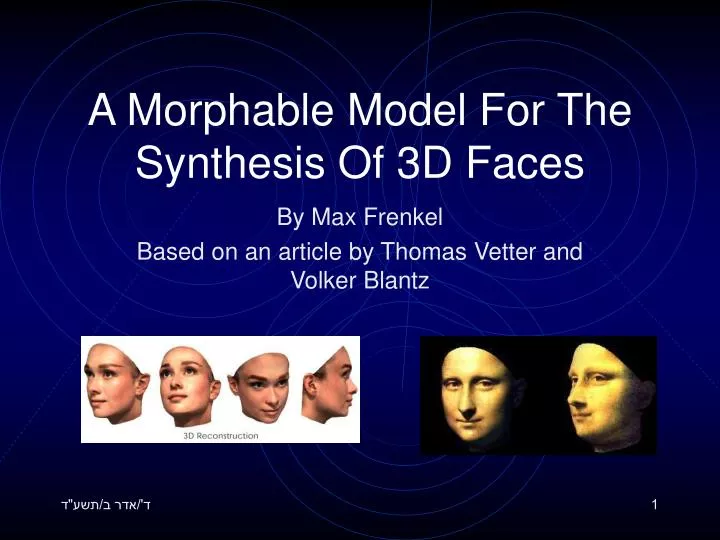
A Morphable Model For The Synthesis Of 3D Faces By Max Frenkel Based on an article by Thomas Vetter and Volker Blantz Introduction The following paper attempts to extend the idea of face models to reconstruct face structure from images taken in less constrained environments. Introduction

E N D
A Morphable Model For The Synthesis Of 3D Faces By Max Frenkel Based on an article by Thomas Vetter and Volker Blantz
Introduction The following paper attempts to extend the idea of face models to reconstruct face structure from images taken in less constrained environments.
Introduction Also, the paper demonstrates an application of facial modeling to facial expression manipulations and generation of new shadows and lighting conditions.
How Do They Do It? By exploiting the statistics of known faces. The structure of newly generated faces is constrained to be in the range of that of known faces.
The Morphable 3D Face Model This time, the actual 3D structure of known faces is captured in the shape vector S = (x1, y1, z1, x2, …, yn, zn)T, containing the (x, y, z) coordinates of the n vertices of a face, and the texture vector T= (R1, G1, B1, R2, …, Gn, Bn)T, containing the color values at the corresponding vertices. Again, assuming that we have m such vector pairs in full correspondence, we can form new shapes Smodel and new textures Tmodel as:
The Morphable 3D Face Model In order to constrain the solution to lie close to our data cloud, we fit a normal distribution to a set of 200 sample faces, using PCA. For shape, we compute the average vector Sav of {Si}i=1..m, offset the data set to the origin: {DSi = Si - Sav}i=1..m, and compute the covariance matrix CS = AS(AS)T, where:
The Morphable 3D Face Model The eigenvalues si2 of CS represent the variance of the data set along the direction si, the corresponding eigenvector of CS. So Smodel can now be expressed as: and the probability density fit over our data set is a function of a = (a1, a2, ... , am)T:
Matching a Morphable Model to Images • Rough initial manual alignment • Reconstruction of 3D shape, texture and rendering parameters – fitting the model to image • Extracting texture from image
Fitting the Model to an Image • Coefficients of the 3D model (a1, a2, ... , am)T and (b1, b2, ... , bm)T are optimized together with the rendering parameters r such as camera position, object scale, image plane rotation and translation, intensity of ambient and directed light, etc.
Fitting the Model to an Image • At every iteration the algorithm renders an image Imodel using the current parameters a, b, andr and updates them so as to minimize the residual norm summed over the pixels (x,y) where Iinput is the input image. • Rendering is performed using perspective projection and Phong shading. Projection maps the 3D coordinates of the face model to pixel locations (x,y) in the above norm and the shading algorithm computes the color values at those pixels
Fitting the Model to an Image • To force the set of solutions to lie as close as possible to the means of a, b, andr - the parameters in the database, we maximize the posterior probability p(a, b, r) given Iinput. The distributions are assumed to be Gaussian as mentioned. Thus, we strive to maximize the product p(a) p(b) p(r).
Fitting the Model to an Image • Also, the noise in Iinput is assumed to be Gaussian with variance sN2, so the distribution of the differences between the rendered model and the image at the pixels is modeled as and this term is multiplied into p(a) p(b) p(r).
Fitting the Model to an Image • Maximizing the above product is equivalent to minimizing the log likelihood function after taking the logarithm and flipping the sign. Here, sS,i and sT,i are the standard deviations for shape and texture obtained through PCA as previously mentioned.
Fitting the Model to an Image • The partials E/ai, E/bi, E/ri can be analytically obtained from the above likelihood formulation and the steepest descent procedure can be used to update the parameters at each iteration. Thus, for shape parameters a, we would take steps as follows:
Fitting the Model to an Image • The above procedure is performed on a subset of the vertices of the 3D model. The 3D model is subdivided into triangular patches, and a random subset of the triangles is selected to be processed at each iteration. • The 3D coordinates of the center of each triangle are projected onto the image plane to (x, y), the corresponding intensity Imodel(x, y) is computed, and used in the residual equation
Fitting the Model to an Image A coarse-to-fine strategy is employed. • The first iterations are performed on a subsampled Iinput and a low resolution model. • The highest principal components are used at first, and more are added later on. • Towards the end, the model is broken into segments (similarly to the previous paper) and the parameters are optimized separately for each segment achieving finer resolution.
Texture Extraction • After the shape, texture and illumination parameters are obtained, we can extract the residual at each pixel (x, y) and compute the change in texture required to account for the difference.
Facial Attributes Several classes of attributes are modeled: • Facial expressions (smile, frown) • Individual characteristics (double chin, hooked nose, ‘maleness’) • Distinctiveness
Facial Attributes • Facial expressions For each face in the database, two scans are recorded: Sneutral, and Sexpression. The difference vector DS =Sexpression - Sneutral is saved and later on simply added to the 3D reconstruction of the input image.
Facial Attributes • Individual characteristics For each face in the database, we manually assign labels mi that reflect how much of a certain characteristic is present in a given face (Si, Ti). Then the characteristic DS is obtained from summing up:
Facial Attributes • Distinctiveness Caricatures of faces can be obtained by exaggerating their distinctive features. Once the 3D structure of a face is known and thus a face is positioned in face-space, its distance from the mean of our data cloud can be increased by scaling a, and b.
Building a Morphable Model • In order to build a model out of the faces in the database, they first need to be set in correspondence. • Similarly to the way images are represented as I(x, y) = (R(x, y), G(x, y), B(x, y)), 3D laser scans can be represented in cylindrical coordinates as I(h, f) = (R(h, f), G(h, f), B(h, f), r(h, f)), where f is the pitch angle, h is the height, and r is the radius.
Building a Morphable Model • Now, the correspondence problem is to compute a flow field (dh(h, f), df(h, f)) that minimizes • The above norm is minimized by taking small windows around each ‘pixel’ and assuming that the flow vector is constant per window. • The problem is solved on multiple levels of resolution to avoid local minima.
Summary and Results • 200 3D scans were taken and set in correspondence using the described optical flow technique. • Using PCA, the first 100 principal components of the model were used to fit it to new faces. • Images of arbitrary Caucasian faces of middle age were either taken with a digital camera or taken under unknown conditions.
Summary and Results • After rough manual initialization, a gradient descent technique minimizes a functional that gives preference to reconstructed faces that are closer to the average face in the database.
Summary and Results • After reconstruction, additional texture is extracted from the input image using the obtained shape, texture, and rendering parameters by looking at the residual at each pixel. • New images are rendered modeling artificial lighting conditions, rotations, and facial attributes
Summary and Results • 3D reconstruction given a single image is an ill-posed problem, however, to human observers who know only the input image, the results look correct.