Download
1 / 59
590 likes | 830 Views
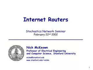
Internet Routers Stochastics Network Seminar February 22 nd 2002. Nick McKeown Professor of Electrical Engineering and Computer Science, Stanford University nickm@stanford.edu www.stanford.edu/~nickm. What a Router Looks Like. Cisco GSR 12416. Juniper M160. 19”. 19”.

E N D
Internet Routers Stochastics Network Seminar February 22nd 2002 Nick McKeown Professor of Electrical Engineering and Computer Science, Stanford University nickm@stanford.edu www.stanford.edu/~nickm
What a Router Looks Like Cisco GSR 12416 Juniper M160 19” 19” Capacity: 160Gb/sPower: 4.2kW Capacity: 80Gb/sPower: 2.6kW 6ft 3ft 2ft 2.5ft
POP3 POP2 POP1 D POP4 A B E POP5 POP6 C POP7 POP8 F Points of Presence (POPs)
Basic Architectural Componentsof an IP Router Routing Protocols Control Plane Routing Table Datapath per-packet processing Forwarding Table Switching
Per-packet processing in an IP Router 1. Accept packet arriving on an ingress line. 2. Lookup packet destination address in the forwarding table, to identify outgoing interface(s). 3. Manipulate packet header: e.g., decrement TTL, update header checksum. 4. Send packet to outgoing interface(s). 5. Queue until line is free. 6. Transmit packet onto outgoing line.
Data Hdr Data Hdr IP Address Next Hop Address Table Buffer Memory ~1M prefixes Off-chip DRAM ~1M packets Off-chip DRAM Generic Router Architecture Header Processing Lookup IP Address Update Header Queue Packet
Header Processing Header Processing Header Processing Lookup IP Address Lookup IP Address Lookup IP Address Update Header Update Header Update Header Address Table Address Table Address Table Generic Router Architecture Buffer Manager Buffer Memory Buffer Manager Buffer Memory Buffer Manager Buffer Memory
Packet processing is getting harder CPU Instructions per minimum length packet since 1996
WFQ Performance metrics • Capacity • “maximize C, s.t. volume < 2m3 and power < 5kW” • Throughput • Operators like to maximize usage of expensive long-haul links. • This would be trivial with work-conserving output-queued routers • Controllable Delay • Some users would like predictable delay. • This is feasible with output-queueing plus weighted fair queueing (WFQ).
Can’t I just use N separate memory devices per output? output 1 R R R R N The Problem • Output queued switches are impractical R R R R DRAM data NR NR
Memory BandwidthCommercial DRAM • It’s hard to keep up with Moore’s Law: • The bottleneck is memory speed. • Memory speed is not keeping up with Moore’s Law. DRAM 1.1x / 18months Moore’s Law 2x / 18 months Router Capacity 2.2x / 18months Line Capacity 2x / 7 months
Header Processing Header Processing Header Processing Lookup IP Address Lookup IP Address Lookup IP Address Update Header Update Header Update Header Address Table Address Table Address Table Generic Router Architecture Queue Packet 1 1 Buffer Memory 2 2 Queue Packet Buffer Memory Scheduler Queue Packet N N Buffer Memory
Outline of next two talks • What’s known about throughput • Today: Survey of ways to achieve 100% throughput • What’s known about controllable delay • Next week (Sundar): Controlling delay in routers with a single stage of buffering.
Potted history • [Karol et al. 1987] Throughput limited to by head-of-line blocking for Bernoulli IID uniform traffic. • [Tamir 1989] Observed that with “Virtual Output Queues” (VOQs) Head-of-Line blocking is reduced and throughput goes up.
Potted history • [Anderson et al. 1993] Observed analogy to maximum size matching in a bipartite graph. • [M et al. 1995] (a) Maximum size match can not guarantee 100% throughput.(b) But maximum weight match can – O(N3). • [Mekkittikul and M 1998] A carefully picked maximum size match can give 100% throughput. Matching O(N2.5)
Potted history Speedup 5. [Chuang, Goel et al. 1997] Precise emulation of a central shared memory switch is possible with a speedup of two and a “stable marriage” scheduling algorithm. • [Prabhakar and Dai 2000] 100% throughput possible for maximal matching with a speedup of two.
Potted historyNewer approaches • [Tassiulas 1998] 100% throughput possible for simple randomized algorithm with memory. • [Giaccone et al. 2001] “Apsara” algorithms. • [Iyer and M 2000] Parallel switches can achieve 100% throughput and emulate an output queued switch. • [Chang et al. 2000] A 2-stage switch with a TDM scheduler can give 100% throughput. • [Iyer, Zhang and M 2002] Distributed shared memory switches can emulate an output queued switch.
Scheduling crossbar switches to achieve 100% throughput • Basic switch model. • When traffic is uniform (Many algorithms…) • When traffic is non-uniform, but traffic matrix is known. • Technique: Birkhoff-von Neumann decomposition. • When matrix is not known. • Technique: Lyapunov function. • When algorithm is pipelined, or information is incomplete. • Technique: Lyapunov function. • When algorithm does not complete. • Technique: Randomized algorithm. • When there is speedup. • Technique: Fluid model. • When there is no algorithm. • Technique: 2-stage load-balancing switch. • Technique: Parallel Packet Switch.
Basic Switch Model S(n) L11(n) A11(n) 1 1 D1(n) A1(n) A1N(n) AN1(n) DN(n) AN(n) N N ANN(n) LNN(n)
Some definitions 3. Queue occupancies: Occupancy L11(n) LNN(n)
Some definitions of throughput When traffic is admissible
Scheduling algorithms to achieve 100% throughput • Basic switch model. • When traffic is uniform (Many algorithms…) • When traffic is non-uniform, but traffic matrix is known • Technique: Birkhoff-von Neumann decomposition. • When matrix is not known. • Technique: Lyapunov function. • When algorithm is pipelined, or information is incomplete. • Technique: Lyapunov function. • When algorithm does not complete. • Technique: Randomized algorithm. • When there is speedup. • Technique: Fluid model. • When there is no algorithm. • Technique: 2-stage load-balancing switch. • Technique: Parallel Packet Switch.
Algorithms that give 100% throughput for uniform traffic • Quite a few algorithms give 100% throughput when traffic is uniform1 • For example: • Maximum size bipartite match. • Maximal size match (e.g. PIM, iSLIP, WFA) • Deterministic and a few variants • Wait-until-full 1. “Uniform”: the destination of each cell is picked independently and uniformly and at random (uar) from the set of all outputs.
Maximum size bipartite match • Intuition: maximizes instantaneous throughput • for uniform traffic. L11(n)>0 Maximum Size Match LN1(n)>0 Bipartite Match “Request” Graph
Aside: Maximal Matching • A maximal matching is one in which each edge is added one at a time, and is not later removed from the matching. • i.e. no augmenting paths allowed (they remove edges added earlier). • No input and output are left unnecessarily idle.
Aside: Example of Maximal Size Matching A 1 A 1 2 B 2 B 3 C 3 C 4 4 D D 5 5 E E 6 6 F F Maximum Matching Maximal Matching
Algorithms that give 100% throughput for uniform traffic • Quite a few algorithms give 100% throughput when traffic is uniform • For example: • Maximum size bipartite match. • Maximal size match (e.g. PIM, iSLIP, WFA) • Determinstic and a few variants • Wait-until-full
Deterministic Scheduling Algorithm If arriving traffic is i.i.d with destinations picked uar across outputs, then a round-robin schedule gives 100% throughput. A 1 A 1 A 1 2 2 B B 2 B 3 3 C C 3 C 4 4 D D 4 D Variation 1: if permutations are picked uar from the set of N! permutations, this too will also give 100% throughput. Variation 2: if permutations are picked uar from the permutations above, this too will give 100% throughput.
A Simple wait-until-full algorithm • The following algorithm appears to be stable for Bernoulli i.i.d. uniform arrivals: • If any VOQ is empty, do nothing (i.e. serve no queues). • If no VOQ is empty, pick a permutation uar across either (sequence of permutations, or all permutations).
Some observations • A maximum size match (MSM) maximizes instantaneous throughput. • But a MSM is complex – O(N2.5). • It turns out that there are many simple algorithms that give 100% throughput for uniform traffic. • So what happens if the traffic is non-uniform?
Why doesn’t maximizing instantaneous throughput give 100% throughput for non-uniform traffic? Three possible matches, S(n):
Scheduling algorithms to achieve 100% throughput • Basic switch model. • When traffic is uniform (Many algorithms…) • When traffic is non-uniform, but traffic matrix is known • Technique: Birkhoff-von Neumann decomposition. • When matrix is not known. • Technique: Lyapunov function. • When algorithm is pipelined, or information is incomplete. • Technique: Lyapunov function. • When algorithm does not complete. • Technique: Randomized algorithm. • When there is speedup. • Technique: Fluid model. • When there is no algorithm. • Technique: 2-stage load-balancing switch. • Technique: Parallel Packet Switch.
Example 1: (Trivial) scheduling to achieve 100% throughput • Assume we know the traffic matrix, and the arrival pattern is deterministic: • Then we can simply choose:
Example 2:With random arrivals, but known traffic matrix • Assume we know the traffic matrix, and the arrival pattern is random: • Then we can simply choose: • In general, if we know L, can we pick a sequence S(n) to achieve 100% throughput?
Birkhoff - von Neumann Decomposition Any L can be decomposed into a linear (convex) combination of matrices, (M1, …, Mr).
In practice… • Unfortunately, we usually don’t know traffic matrix La priori, so we can: • Measure or estimate L, or • Not use L. • In what follows, we will assume we don’t know or use L.
Scheduling algorithms to achieve 100% throughput • Basic switch model. • When traffic is uniform (Many algorithms…) • When traffic is non-uniform, but traffic matrix is known • Technique: Birkhoff-von Neumann decomposition. • When traffic matrix is not known. • Technique: Lyapunov function. • When algorithm is pipelined, or information is incomplete. • Technique: Lyapunov function. • When algorithm does not complete. • Technique: Randomized algorithm. • When there is speedup. • Technique: Fluid model. • When there is no algorithm. • Technique: 2-stage load-balancing switch. • Technique: Parallel Packet Switch.
Maximum weight matching S*(n) L11(n) A11(n) A1(n) D1(n) 1 1 A1N(n) AN1(n) AN(n) DN(n) ANN(n) N N LNN(n) L11(n) Maximum Weight Match LN1(n) Bipartite Match “Request” Graph
Scheduling algorithms to achieve 100% throughput • Basic switch model. • When traffic is uniform (Many algorithms…) • When traffic is non-uniform, but traffic matrix is known. • Technique: Birkhoff-von Neumann decomposition. • When matrix is not known. • Technique: Lyapunov function. • When algorithm is pipelined, or information is incomplete. • Technique: Lyapunov function. • When algorithm does not complete. • Technique: Randomized algorithm. • When there is speedup. • Technique: Fluid model. • When there is no algorithm. • Technique: 2-stage load-balancing switch. • Technique: Parallel Packet Switch.
Scheduling algorithms to achieve 100% throughput • Basic switch model. • When traffic is uniform (Many algorithms…) • When traffic is non-uniform, but traffic matrix is known. • Technique: Birkhoff-von Neumann decomposition. • When matrix is not known. • Technique: Lyapunov function. • When algorithm is pipelined, or information is incomplete. • Technique: Lyapunov function. • When algorithm does not complete. • Technique: Randomized algorithm. • When there is speedup. • Technique: Fluid model. • When there is no algorithm. • Technique: 2-stage load-balancing switch. • Technique: Parallel Packet Switch.
Achieving 100% when algorithm does not complete Randomized algorithms: • Basic idea (Tassiulas) • Reducing delay (Shah, Giaccone and Prabhakar)
Scheduling algorithms to achieve 100% throughput • Basic switch model. • When traffic is uniform (Many algorithms…) • When traffic is non-uniform, but traffic matrix is known. • Technique: Birkhoff-von Neumann decomposition. • When matrix is not known. • Technique: Lyapunov function. • When algorithm is pipelined, or information is incomplete. • Technique: Lyapunov function. • When algorithm does not complete. • Technique: Randomized algorithm. • When there is speedup. • Technique: Fluid model. • When there is no algorithm. • Technique: 2-stage load-balancing switch. • Technique: Parallel Packet Switch.