Download
1 / 53
540 likes | 990 Views
Estimating the Laplace-Beltrami Operator by Restricting 3D Functions Ming Chuang 1 , Linjie Luo 2 , Benedict Brown 3 , Szymon Rusinkiewicz 2 , and Misha Kazhdan 1 1 Johns Hopkins University 3 Katholieke Universiteit Leuven 2 Princeton University Motivation Image Stitching

E N D
Estimating the Laplace-Beltrami Operator by Restricting 3D Functions • Ming Chuang1, Linjie Luo2, Benedict Brown3,Szymon Rusinkiewicz2, and Misha Kazhdan1 1Johns Hopkins University • 3KatholiekeUniversiteit Leuven 2Princeton University
Motivation Image Stitching • Compute image gradients • Set seam-crossing gradients to zero • Fit image to the new gradient field
Motivation Gradient-Domain Image Processing Solving for the scalar field u whose gradients best match the vector field g amounts to solving a Poisson system: This approach is popular in image-processing because multigrid makes solving the system simple and fast. Can the analog on meshes also be made easy to implement?
Outlook To address this question, we consider two related problems: • How to define the Laplace-Beltrami operator. • How to implement a hierarchical solver.
Outlook To address this question, we consider two related problems: • How to define the Laplace-Beltrami operator. • How to implement a hierarchical solver. Impose regular structure byrestricting functions definedon a voxel grid
Outline • Introduction • Review • Defining the system • Solving the system • Our Approach • Results • Discussion of Limitations • Conclusion and Future Work
Defining the System Finite Elements (Galerkin) Define a set of test functions {b1,…,bn} and discretize the problem: if appropriate boundary conditions are met. When n test functions are used, this results in an nxn system: where L is the Laplacian matrix:and y is the constraint vector:
Solving the System Multigrid Solvers • Relax the system at the finest resolution • Down-sample the residual • Solve at the coarser resolution • Up-sample the coarse correction • Relax the system at the finest resolution Relax Relax Up-Sample Down-Sample Solve
Solving the System Multigrid Solvers • Relax the system at the finest resolution • Down-sample the residual • Solve at the coarser resolution • Up-sample the coarse correction • Relax the system at the finest resolution Relaxation: Gauss-Seidel Solver: Recurse/direct-solve Up/Down-Sampling: ??? Relax Relax Up-Sample Down-Sample Solve
Defining the System (Regular Grids) In one dimension, use translates of B-splines: In higher dimensions, usetranslates of tensor-products: … … bi-1(x) bi(x) bi+1(x) b(x) 1.5 -1.5 (i,j) bi(x) bj(y)
Up/Down-Sampling (Regular Grids) Use the fact that the B-splines nest, so that coarser elements can be expressed as linear combinations of finer elements: 3/4 3/4 1/4 1/4
Defining the System (Meshes) Associate a function with each vertex and use the span to define a function space. bi(p) When the bi(p) are hat functions, we get the cotangent-weight Laplacian: pi pi-1 pi+1 pi pk bi(p) pj
Up/Down-Sampling (Meshes) Define a coarser surface/graph and amapping from the coarser topologyinto the finer: • Geometric Multigrid [Kobbeltet al., 1998] [Ray and Lévy, 2003][Aksolyuet al., 2005] [Ni et al., 2004] • Algebraic Multigrid [Ruge and Stueben, 1987] [Cleary et al., 2000][Brezinaet al., 2000] [Chartieret al. 2003][Shi et al., 2006]
Outline • Introduction • Review • Our Approach • Key Idea • Implementation • Results • Discussion of Limitations • Conclusion and Future Work
Our Approach Key Idea Start with elements defined over a regular grid, and only consider the restriction to the surface. bi(x) bj(y)
Our Approach Key Idea Start with elements defined over a regular grid, and only consider the restriction to the surface. Properties • Tesselation IndependenceThe definition onlydepends on the position ofpoints on the surface bi(x) bj(y)
Our Approach Key Idea Start with elements defined over a regular grid, and only consider the restriction to the surface. Properties • Tesselation Independence • Multi-resolution hierarchyNested spaces remain nested after restriction
Our Approach Implementation We must address three concerns: • Define the system • Index the elements • Solve with multigrid
Our Approach Defining the System Given elements {b1,…,bn} defined on a regular grid, we define the coefficients of the Laplace-Beltrami operator as integrals of gradients:
Our Approach Defining the System Given elements {b1,…,bn} defined on a regular grid, we define the coefficients of the Laplace-Beltrami operator as integrals of gradients: When M={T1,…,Tm}, the coefficients of the Laplace-Beltrami operator can be expressed as:
Defining the System Computing the Integrals • Explicit Integration • Approximate Integration
Defining the System Computing the Integrals • Explicit IntegrationB-splines are strictly polynomial within a cell, so split the triangles to the grid and integrate the over the split triangles. [Taylor, 2008]
Defining the System Computing the Integrals • Explicit Integration • Approximate IntegrationSample the surface and approximate the integral as a sum over the oriented point-set.
Indexing the Elements Most elements’ supports do not overlap the surface so their restriction is the zero-function.
Indexing the Elements Most elements’ supports do not overlap the surface so their restriction is the zero-function. Adapted OctreeDiscard all cells whosesupport does not overlapthe shape.
Solving with Multigrid Because the restricted functions remain nested, the up-/down-sampling operators do not change and we can solve just like with regular grids. Relax Relax Up-Sample Down-Sample Solve
Outline • Introduction • Review • Our Approach • Results • Gradient-Domain Processing • Spectral Analysis • Discussion of Limitations • Conclusion and Future Work
Gradient-Domain Processing Goal Given a base mesh and a set of scans, generate a seamless texture on the mesh. S1 S5 M S4 S2 S3
Gradient-Domain Processing Goal Given a base mesh and a set of scans, generate a seamless texture on the mesh. Back-project surface points onto the scans and use data from the closest, consistent scan. S1 S5 M S4 S2 S3
Gradient-Domain Processing Challenge Pulling colors from the nearest scan results in a discontinuous texture. S1 S5 M S4 S2 S3
Gradient-Domain Processing Solution Pulling gradients and integrating gives seamless textures (which are smooth in undefined areas). S1 S5 M S4 S2 S3
Gradient-Domain Processing Complexity • System scales as O(4depth) • Solver is linear in system size/dimension Depth: 4 Dim: 1,576 Solved: <0.1 Depth: 5 Dim: 6,555 Solved: 0.3 (s) Depth: 6 Dim: 26,771 Solved: 1.4 (s) Depth: 7 Dim: 107,690 Solved: 6.6 (s) Depth: 8 Dim: 431,859 Solved: 28.5 (s)
Gradient-Domain Processing Comparison with AMG (Residual Ratio of 10-3) • AMG1 Classical AMG [Ruge and Stueben, 1987] • AMG2 BoomerAMG[Griebelet al., 2006] AMG1:AMG2:Ours: 0.5 (s) 0.4 (s)0.1 (s) AMG1: AMG2:Ours: 10.9 (s) 4.0 (s)2.6 (s) AMG1:AMG2: Ours: 3.6 (s) 1.6 (s)0.9 (s) AMG1: AMG2:Ours: 34.5 (s) 12.3 (s)7.6 (s) AMG1: AMG2:Ours: 100.1 (s) 36.2 (s)20.8 (s)
Spectral Analysis We can measure the quality of our Laplace-Beltrami operator by evaluating its spectrum.
Spectral Analysis (Sphere) We can measure the quality of our Laplace-Beltrami operator by evaluating its spectrum. For a sphere, eigenvalues come in groups, with: • (2l+1) eigenvectors inthe l-th group, and • all vectors in thel-th group havingeigenvaluel(l+1) True
Spectral Analysis (Sphere) Computing the spectra of the Cotangent-Weight Laplace-Beltrami operator on a coarse mesh, we can lose accuracy at high frequencies. Dim = 2,562 True Cotangent (coarse)
Spectral Analysis (Sphere) Refining the tesselation, we can obtain a more accurate spectrum at the cost of a larger system. Dim = 2,562 Dim = 10,242 True Cotangent (coarse) Cotangent (fine)
Spectral Analysis (Sphere) Using our Laplace-Beltrami operator, we obtain a more accurate spectrum from a matrix that is independent of the tesselation. Dim = 2,562 Dim = 10,242 Dim = 2,832 True Cotangent (coarse) Cotangent (fine) Ours
Spectral Analysis (Sphere) Using our Laplace-Beltrami operator, we obtain a more accurate spectrum from a matrix that is independent of the tesselation. Dim = 2,562 Dim = 10,242 Dim = 2,832 True Cotangent (coarse) Cotangent (fine) Ours
Spectral Analysis (Fish) When the true spectrum is not known, we can compare against the spectrum of the Cotangent-Weight operator at a fine tesselation. Dim = 3,700 Dim = 14,800 Dim = 3,619 “True” (59,200) Cotangent (coarse) Cotangent (fine) Ours
Spectral Analysis (Pulley) When the true spectrum is not known, we can compare against the spectrum of the Cotangent-Weight operator at a fine tesselation. Dim = 6,459 Dim = 19,499 Dim = 6,160 “True” (45,676) Cotangent (coarse) Cotangent (fine) Ours
Limitations • Euclidean vs. Geodesic proximity • Poor Conditioning
Limitations • Euclidean vs. Geodesic proximity • Poor Conditioning
Limitations • Euclidean vs. Geodesic proximity • Poor Conditioning
Outline • Introduction • Review • Our Approach • Results • Discussion of Limitations • Conclusion and Future Work
Conclusion Considered a representation of finite elements on meshes that are defined over a regular grid: • Tesselation invariant Laplace-Beltrami • Regularly indexed elements • Multigrid without remeshing • Simple up-/down-sampling
Future Work Implementation • Parallelize Solvers • Stream Solvers Applications • Deformation • Surface Reconstruction Address Limitations • Duplicate nodes for disconnected components • Use WEB-splines for handling ill-conditioning
Gradient-Domain Processing Convergence Using large point samples allows for accurate linear systems with much lower set-up time. 255 0 Points: 105 Set-Up: 10(s) Points: 106 Set-Up: 14(s) Points: 107 Set-Up: 49(s) Points: Set-Up: 786(s) Points: 104 Set-Up: 9(s) Dimension: 1.1-1.4 x 10⁵ Solve: 5-6 (s)