Download
1 / 77
810 likes | 1.24k Views
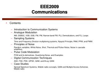
EEE2009 Communications. Contents Introduction to Communication Systems Analogue Modulation AM, DSBSC, VSB, SSB, FM, PM, Narrow band FM, PLL Demodulators, and FLL Loops Sampling Systems Time and Frequency Division multiplexing systems, Nyquist Principle, PAM, PPM, and PWM.

E N D
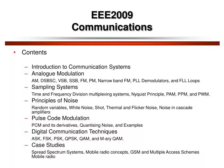
EEE2009Communications • Contents • Introduction to Communication Systems • Analogue Modulation AM, DSBSC, VSB, SSB, FM, PM, Narrow band FM, PLL Demodulators, and FLL Loops • Sampling Systems Time and Frequency Division multiplexing systems, Nyquist Principle, PAM, PPM, and PWM. • Principles of Noise Random variables, White Noise, Shot, Thermal and Flicker Noise, Noise in cascade amplifiers • Pulse Code Modulation PCM and its derivatives, Quantising Noise, and Examples • Digital Communication Techniques ASK, FSK, PSK, QPSK, QAM, and M-ary QAM. • Case Studies Spread Spectrum Systems, Mobile radio concepts, GSM and Multiple Access Schemes Mobile radio
Recommended Text Books • “An introduction to Analogue and Digital communication”, Haykin (Wiley) • “Communication Systems”, Carlson (McGraw & Hill) • “Information, Transmission, Modulation and Noise”, Schwartz (McGraw & Hill) • “Analogue and Digital Communication Systems”, Raden (Prentice-Hall) • “Communication Systems”, Haykin (Wiley) • “Electronic Communication Techniques”, Young (Merril-Publ)
Introduction to Modulation and Demodulation The purpose of a communication system is to transfer information from a source to a destination. • In practice, problems arise in baseband transmissions, • the major cases being: • Noise in the system – external noise • and circuit noise reduces the • signal-to-noise (S/N) ratio at the receiver • (Rx) input and hence reduces the • quality of the output. • Such a system is not able to fully utilise the available bandwidth, • for example telephone quality speech has a bandwidth ≃ 3kHz, a • co-axial cable has a bandwidth of 100's of Mhz. • Radio systems operating at baseband frequencies are very difficult. • Not easy to network.
Multiplexing Multiplexing is a modulation method which improves channel bandwidth utilisation. For example, a co-axial cable has a bandwidth of 100's of Mhz. Baseband speech is a only a few kHz
1) Frequency Division Multiplexing FDM This allows several 'messages' to be translated from baseband, where they are all in the same frequency band, to adjacent but non overlapping parts of the spectrum. An example of FDM is broadcast radio (long wave LW, medium wave MW, etc.)
2) Time Division Multiplexing TDM TDM is another form of multiplexing based on sampling which is a modulation technique. In TDM, samples of several analogue message symbols, each one sampled in turn, are transmitted in a sequence, i.e. the samples occupy adjacent time slots.
Radio Transmission • Aerial dimensions are of the same order as the wavelength, , of the signal • (e.g. quarter wave /4, /2 dipoles). where c is the velocity of an electromagnetic wave, and c = 3x10⁸ m/sec in free space. is related to frequency by = 105 metres or 100km. For baseband speech, with a signal at 3kHz, (3x10³Hz) • Aerials of this size are impractical although some transmissions at Very Low Frequency (VLF) for specialist • applications are made. • A modulation process described as 'up-conversion' (similar to FDM) allows the baseband signal to be • translated to higher 'radio' frequencies. • Generally 'low' radio frequencies 'bounce' off the ionosphere and travel long distances around the earth, • high radio frequencies penetrate the ionosphere and make space communications possible. • The ability to 'up convert' baseband signals has implications on aerial dimensions and design, long distance • terrestrial communications, space communications and satellite communications. Background 'radio' noise • is also an important factor to be considered. • In a similar content, optical (fibre optic) communications is made possible by a modulation process in which • an optical light source is modulated by an information source.
Networks • A baseband system which is essentially point-to-point could be operated in a network. Some forms of access control (multiplexing) would be desirable otherwise the performance would be limited. Analogue communications networks have been in existence for a long time, for example speech radio networks for ambulance, fire brigade, police authorities etc. • For example, 'digital speech' communications, in which the analogue speech signal is converted to a digital signal via an analogue-to-digital converter give a form more convenient for transmission and processing.
What is Modulation? In modulation, a message signal, which contains the information is used to control the parameters of a carrier signal, so as to impress the information onto the carrier. The Messages The message or modulating signal may be either: analogue – denoted by m(t) digital – denoted by d(t) – i.e. sequences of 1's and 0's The message signal could also be a multilevel signal, rather than binary; this is not considered further at this stage. The Carrier The carrier could be a 'sine wave' or a 'pulse train'. Consider a 'sine wave' carrier: • If the message signal m(t) controls amplitude – gives AMPLITUDE MODULATION AM • If the message signal m(t) controls frequency – gives FREQUENCY MODULATION FM • If the message signal m(t) controls phase- gives PHASE MODULATION PM or M
Considering now a digital message d(t): • If the message d(t) controls amplitude – gives AMPLITUDE SHIFT KEYING ASK. • As a special case it also gives a form of Phase Shift Keying (PSK) called PHASE REVERSAL • KEYING PRK. • If the message d(t) controls frequency – gives FREQUENCY SHIFT KEYING FSK. • If the message d(t) controls phase – gives PHASE SHIFT KEYING PSK. • In this discussion, d(t) is a binary or 2 level signal representing 1's and 0's • The types of modulation produced, i.e. ASK, FSK and PSK are sometimes described as binary • or 2 level, e.g. Binary FSK, BFSK, BPSK, etc. or 2 level FSK, 2FSK, 2PSK etc. • Thus there are 3 main types of Digital Modulation: • ASK, FSK, PSK.
Multi-Level Message Signals As has been noted, the message signal need not be either analogue (continuous) or binary, 2 level. A message signal could be multi-level or m levels where each level would represent a discrete pattern of 'information' bits. For example, m = 4 levels
In general n bits per codeword will give 2n = m different patterns or levels. • Such signals are often called m-ary (compare with binary). • Thus, with m = 4 levels applied to: • Amplitude gives 4ASK or m-ary ASK • Frequency gives 4FSK or m-ary FSK • Phase gives 4PSK or m-ary PSK 4 level PSK is also called QPSK (Quadrature Phase Shift Keying).
Consider Now A Pulse Train Carrier where and • The 3 parameters in the case are: • Pulse Amplitude E • Pulse width vt • Pulse position T • Hence: • If m(t) controls E – gives PULSE AMPLITUDE MODULATION PAM • If m(t) controls t - gives PULSE WIDTH MODULATION PWM • If m(t) controls T - gives PULSE POSITION MODULATION PPM • In principle, a digital message d(t) could be applied but this will not be considered further.
What is Demodulation? Demodulation is the reverse process (to modulation) to recover the message signal m(t) or d(t) at the receiver.
Summary of Modulation Techniques with some Derivatives and Familiar Applications
Summary of Modulation Techniques with some Derivatives and Familiar Applications
Summary of Modulation Techniques with some Derivatives and Familiar Applications 2
Analogue Modulation – Amplitude Modulation Consider a 'sine wave' carrier. vc(t) = Vc cos(ct), peak amplitude = Vc, carrier frequency c radians per second. Since c = 2fc, frequency = fc Hz where fc = 1/T. Amplitude Modulation AM In AM, the modulating signal (the message signal) m(t) is 'impressed' on to the amplitude of the carrier.
Message Signal m(t) In general m(t) will be a band of signals, for example speech or video signals. A notation or convention to show baseband signals for m(t) is shown below
Message Signal m(t) In general m(t) will be band limited. Consider for example, speech via a microphone. The envelope of the spectrum would be like:
Message Signal m(t) In order to make the analysis and indeed the testing of AM systems easier, it is common to make m(t) a test signal, i.e. a signal with a constant amplitude and frequency given by
Schematic Diagram for Amplitude Modulation VDC is a variable voltage, which can be set between 0 Volts and +V Volts. This schematic diagram is very useful; from this all the important properties of AM and various forms of AM may be derived.
Equations for AM From the diagram where VDC is the DC voltage that can be varied. The equation is in the form Amp cos ct and we may 'see' that the amplitude is a function of m(t) and VDC. Expanding the equation we get:
Equations for AM Now let m(t) = Vmcos mt, i.e. a 'test' signal, Using the trig identity we have Components: Carrier upper sideband USB lower sideband LSB Amplitude:VDCVm/2 Vm/2 Frequency:cc + mc – m fc fc + fm fc + fm This equation represents Double Amplitude Modulation – DSBAM
Spectrum and Waveforms The following diagrams represent the spectrum of the input signals, namely (VDC + m(t)), with m(t) = Vmcos mt, and the carrier cos ct and corresponding waveforms.
Spectrum and Waveforms The above are input signals. The diagram below shows the spectrum and corresponding waveform of the output signal, given by
Double Sideband AM, DSBAM The component at the output at the carrier frequency fc is shown as a broken line with amplitude VDC to show that the amplitude depends on VDC. The structure of the waveform will now be considered in a little more detail. Waveforms Consider again the diagram VDC is a variable DC offset added to the message; m(t) = Vm cos mt
Double Sideband AM, DSBAM This is multiplied by a carrier, cos ct. We effectively multiply (VDC + m(t)) waveform by +1, -1, +1, -1, ... The product gives the output signal
Modulation Depth Consider again the equation , which may be written as The ratio is Modulation Depth defined as the modulation depth, m, i.e. From an oscilloscope display the modulation depth for Double Sideband AM may be determined as follows:
Modulation Depth 2 2Emax = maximum peak-to-peak of waveform 2Emin = minimum peak-to-peak of waveform Modulation Depth This may be shown to equal as follows: = =
Double Sideband Modulation 'Types' There are 3 main types of DSB • Double Sideband Amplitude Modulation, DSBAM – with carrier • Double Sideband Diminished (Pilot) Carrier, DSB Dim C • Double Sideband Suppressed Carrier, DSBSC • The type of modulation is determined by the modulation depth, which for a fixed m(t) depends on the DC offset, VDC. Note, when a modulator is set up, VDC is fixed at a particular value. In the following illustrations we will have a fixed message, Vm cos mt and vary VDC to obtain different types of Double Sideband modulation.
Graphical Representation of Modulation Depth and Modulation Types.
Graphical Representation of Modulation Depth and Modulation Types 2.
Graphical Representation of Modulation Depth and Modulation Types 3 Note then that VDCmay be set to give the modulation depth and modulation type. DSBAM VDC >> Vm, m 1 DSB Dim C 0 < VDC < Vm, m > 1 (1 < m < ) DSBSC VDC = 0, m = The spectrum for the 3 main types of amplitude modulation are summarised
Bandwidth Requirement for DSBAM In general, the message signal m(t) will not be a single 'sine' wave, but a band of frequencies extending up to B Hz as shown Remember – the 'shape' is used for convenience to distinguish low frequencies from high frequencies in the baseband signal.
Bandwidth Requirement for DSBAM Amplitude Modulation is a linear process, hence the principle of superposition applies. The output spectrum may be found by considering each component cosine wave in m(t) separately and summing at the output. Note: • Frequency inversion of the LSB • the modulation process has effectively shifted or frequency translated the baseband m(t) message signal to USB and LSB signals centred on the carrier frequency fc • the USB is a frequency shifted replica of m(t) • the LSB is a frequency inverted/shifted replica of m(t) • both sidebands each contain the same message information, hence either the LSB or USB could be removed (because they both contain the same information) • the bandwidth of the DSB signal is 2B Hz, i.e. twice the highest frequency in the baseband signal, m(t) • The process of multiplying (or mixing) to give frequency translation (or up-conversion) forms the basis of radio transmitters and frequency division multiplexing which will be discussed later.
Power Considerations in DSBAM Remembering that Normalised Average Power = (VRMS)2 = we may tabulate for AM components as follows: Total Power PT = Carrier Power Pc + PUSB + PLSB
Power Considerations in DSBAM From this we may write two equivalent equations for the total power PT, in a DSBAM signal and or The carrier power i.e. Either of these forms may be useful. Since both USB and LSB contain the same information a useful ratio which shows the proportion of 'useful' power to total power is
Power Considerations in DSBAM For DSBAM (m 1), allowing for m(t) with a dynamic range, the average value of m may be assumed to be m = 0.3 Hence, Hence, on average only about 2.15% of the total power transmitted may be regarded as 'useful' power. ( 95.7% of the total power is in the carrier!) Even for a maximum modulation depth of m = 1 for DSBAM the ratio i.e. only 1/6th of the total power is 'useful' power (with 2/3 of the total power in the carrier).
Example Suppose you have a portable (for example you carry it in your ' back pack') DSBAM transmitter which needs to transmit an average power of 10 Watts in each sideband when modulation depth m = 0.3. Assume that the transmitter is powered by a 12 Volt battery. The total power will be = 444.44 Watts where = 10 Watts, i.e. Hence, total power PT = 444.44 + 10 + 10 = 464.44 Watts. amps! Hence, battery current (assuming ideal transmitter) = Power / Volts = i.e. a large and heavy 12 Volt battery. Suppose we could remove one sideband and the carrier, power transmitted would be 10 Watts, i.e. 0.833 amps from a 12 Volt battery, which is more reasonable for a portable radio transmitter.
Single Sideband Amplitude Modulation One method to produce signal sideband (SSB) amplitude modulation is to produce DSBAM, and pass the DSBAM signal through a band pass filter, usually called a single sideband filter, which passes one of the sidebands as illustrated in the diagram below. The type of SSB may be SSBAM (with a 'large' carrier component), SSBDimC or SSBSC depending on VDC at the input. A sequence of spectral diagrams are shown on the next page.