Download
1 / 32
390 likes | 1.89k Views
Computerized Beer Game. Designing & Managing the Supply Chain Appendix A Youn-Ju Woo. Outline. Introduction The Traditional Beer Game The Scenarios Playing a round Options and Settings Summary. Introduction. Traditional Beer Game

E N D
Computerized Beer Game Designing & Managing the Supply Chain Appendix A Youn-Ju Woo
Outline • Introduction • The Traditional Beer Game • The Scenarios • Playing a round • Options and Settings • Summary
Introduction • Traditional Beer Game • Role-playing simulation of a simple production and distribution system • MIT developed in the 1960s • Computerized Beer Game • Similar to Traditional Beer Game • Possible to test the various SCM concept
The Traditional Beer Game (1) • Retail Manager • Observing external demand • Filling demand as much as possible • Record Back orders • Place order with wholesaler • Factory Manager • Observing demand • Filling demand and back orders • Begins production Demand Card • Distributor Manager • Observing demand • Filling demand and back orders • Place order with factory • Wholesaler Manager • Observing demand • Filling demand and back orders • Place order with distributor
The Traditional Beer Game (2) • Goal of Team • Minimize : Total cost = Holding cost + Shortage cost • Game Rules • Back-order should be filled ASPS • Each manager has only local information • 25 ~50 weeks • Holding cost $0.50, Shortage cost $1 • End of the game • Players are asked to estimate customer demand • The demand information is opened to players • Demand is 4 during the 4 weeks and 8 during the last
The Traditional Beer Game (3) • Difficulties • The students focus on correctly following the rules, not developing an effective strategy • Demand pattern does not reflect a realistic supply chain scenario • Doesn’t demonstrate several important issues in SCM • The real objective is to minimize the total system cost, not individual performance Shortening cycle times and centralizing information are useful The computerized Beer Game isdeveloped
The Scenarios (1) • A simplified beer supply chain • Consist of a single retailer, a single distributor, a single wholesaler and a single factory • Each component has unlimited storage capacity, fixed lead time and order delay time • Every week, each component tries to meet the demand of downstream component • Meet every back order ASPS • No ignore any order • Member orders item to the upstream component Place an order Supplier gets order W W+1 Arrive ordered item W+3
The Scenarios (2) • Other options to model various situations • Lead time reduction, global information sharing, centralized management • A centralized scenario • Factory manager controls the entire supply chain and has information of external demand and entire inventory • Only factory can place orders • Only retailer pays a $4.0 shortage cost
Playing a round (1) • Modeling the first scenario • Player chooses one component (Retailer, Wholesaler, Distributor, Factory) • Computer takes the remaining roles
Playing a round (2) • Order of Events • Step 1 • ◦ Contents of delay 2 moved to delay 1 • Step 2 • ◦ Order from downstream facility are filled • ◦Order = current order + back orders • ◦ Remaining orders = current inventory – Order • Back orders • ◦ Except the retailer, the orders are filled to the delay 2 location of the downstream • Step 3 • ◦ Total costs = accumulated cost from previous period + shortage and Holding cost • ◦ Holding cost = $ 0.5 ×(Inventory at facility + in transit to the next downstream) • ◦ Shortage cost = $ 1 ×Back orders • Step 4 • ◦ Player input the order quantity, other orders are placed by computer
Playing a round (3) • Understanding the Screen • Example; Distributor • Total cost : Accumulated cost from previous period and shortage and Holding cost • Backorder: Orders received by the Distributor but not yet met from inventory Number of items in inventory In transit to inventory Delay 1: No. of items will arrive in one week
Playing a round (4) 1. Click start Input order quantity Start Button • Week 0 • Initial inventory : 4 unit • Delay 1 : 4 unit • Delay 2 : 4 unit • Week 1 • Inventory : 8 unit • Delay 1 : 4 unit • Delay 2 : 0 unit
Playing a round (5) • 2. Enter a demand amount ( Ex, Input 3) • Make balance inventory holding costs and shortage costs • Check the amount of back order your upstream supplier already has to fill • After entering the quantity, the remaining members play automatically, the screen is updated • Total cost = (4 + 0 + 8) ×$ 0.5 = $ 6
Playing a round (6) • 3. Select Next Round • The upstream supplier will try to meet last period’s order (3) • Enter order 6 • Total cost = $ 6 + (0 + 0 + 12) ×$ 0.5 = $ 12
Playing a round (7) • 3. Select Next Round • Total cost = $ 12 + (0 + 12 + 0) ×$ 0.5 + 18 ×$ 1 = $ 36 • How much order quantity should be entered? • Order = current order + back orders Level of back order at the beginning of this round, before the player attempted to fill downstream orders How much total back order Current level of back order
Options and Settings (1) • File Commands • File-Reset : Reset the game • File-Exit : Exit the game • Options Commands • Options-Player
Options and Settings (2) • Options Commands • Options-Policy • s-S: When inventory falls below s, the system order to bring inventory to S • S-Q: When inventory falls below s, the system places an order for Q • Order to S: Each week, the system order bring inventory to S • Order Q: Each week, the system orders Q • Updated s: The order-up-to level s is updated • - The movingaverage of demand over past 10 wks • - Inventory level falls below s, the system orders up to s, the maximum order size is S • Echelon: A modified version of perododic review echelon policy
Options and Settings (3) • Options - Short Lead Time • Remove delay 2, shorten lead time to 1 week • Option - Centralized • The interactive player manages the factory, can observe external demand and react it • The inventory is only held by Retailer • Option - Demand • Set the external customer demand • Deterministic – Select the constant • demands and weeks • Random Normal – Select Means, • stds, weeks • Option – Global Information • Display iventory and cost information • and external demand at all of the stages
Options and Settings (4) • The Graphs Commands • Graphs - Player • Graphs – Others • Graphs - System
Options and Settings (5) • The Reports Commands • Reports - Player • Reports – Others • Reports - System
Summary Usage of Computerized Beer Game Test the Traditional Beer Game Possible to test the various SCM concept Shortened lead time Centralized SCM SCM with Global information system Setting Various Demand Display Results Graph Report
The Risk Pool Game Designing & Managing the Supply Chain Appendix B Youn-Ju Woo
Outline • Introduction • The Scenarios • Playing several round • Options and Settings • Summary
Introduction • Concept of Risk Pooling • If each retailer maintains separate inventory and safety stock, the higher level of inventory is needed than using pooling system • Risk Pooling Game • Execute both system simultaneously • A system with risk pooling – Centralized System • A system without risk pooling – Decentralized System • Compare the performances to understand the concept
The Scenarios • Centralized Game • A supplier serves a warehouse, which serves three retailers • Decentralized Game • Three retailers order separately , and supplier ships material directly to each retailer • If the demand is not fulfilled at the time, it is lost. • The goal in both system is to maximize profit Order Retailer Retailer Retailer Retailer Order Retailer Retailer Warehouse Supplier Supplier Supply 2 periods Supply 2 periods Order Supply 4 periods
Playing a round (1) • Description of Screen Allocation to retailers Order from supplier Inventory of retailers Cost of goods sold Inventory at least 4 period away from retailers Holding Cost = Revenue – (COGS + Holding) Supplier = Demand met / Total demand * 100
Playing a round (2) Order of Events Step 1. Step 2. Step 3. Step 4. Step 5. • Centralized System: Four period moves to three periods away, inventory three periods is added to warehouse inventory • Inventory one moved to retailer inventory • Each retailer fills demand as much as possible • Both systems faces the same demand • Centralized System: Enter an order for the supplier or keep the default value • Allocate the warehouse inventory to the retailers • Decentralized System: Enter an order for each retailer or keep the default value • The allocation amount must be less than or equal to the total warehouse inventory • Press Orders button • Orders are filled • Cost, Revenue, and service level is calculated
Options and Settings (1) • Play – Play Options • Initial Conditions • The retailers must have same initial inventory • The transit inventories should be same • Demand • Normal distribution • with mean and standard deviation • The slider control enables to control • the correlation of demand at retailers
Options and Settings (2) • Inventory Policy • Safety Stock policy • - Select order-up-to levels • - Using multipliers by • mean demand and Std. deviation • Weeks of Inventory policy • - A single value multiplied by • mean demand • Cost • Holding cost, Cost, and Revenue cost • are per item per period
Options and Settings (3) • The Reports Commands • Reports - Orders • Reports – Demands