Download

1 / 77
930 likes | 1.9k Views
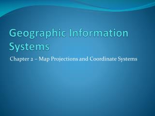
Geographic Information Systems Applications in Natural Resource Management. Chapter 2 GIS Databases: Map Projections, Structures, and Scale. Michael G. Wing & Pete Bettinger. Chapter 2 Objectives. Definition of a map projection, and the components that comprise a projection

E N D
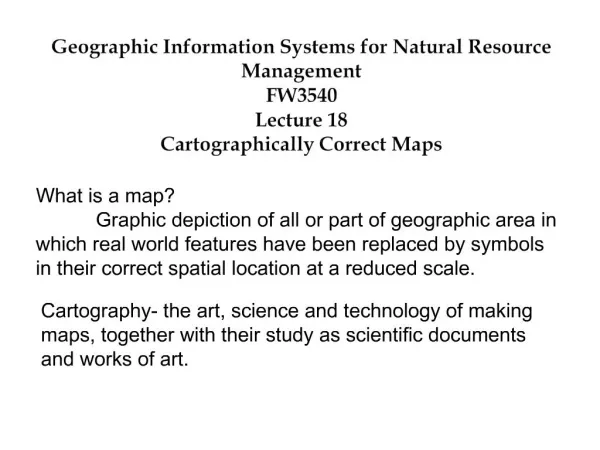
Geographic Information SystemsApplications in Natural Resource Management Chapter 2 GIS Databases: Map Projections, Structures, and Scale Michael G. Wing & Pete Bettinger
Chapter 2 Objectives • Definition of a map projection, and the components that comprise a projection • Components and characteristics of a raster data structure • Components and characteristics of a vector data structure • The purpose and structure of metadata • Likely sources of GIS databases that describe natural resources within North America • Types of information available on a typical topographic map and • Definition of scale and resolution as they relate to GIS databases
Big questions… • What is the size and shape of the earth? • Geodesy: the science of measurements that account for the curvature of the earth and gravitational forces • We are still refining our approximation of the earth’s shape but are relying on GPS measurements for much of this work
Vertical Alexandria Rays parallel to the sun 712’ Earth Syene 712’ 360 / 712’ = 1/50 500 miles * 50 = 25,000 Figure 2.1. Eratosthenes’ (276-194 BC) approach to determining the Earth’s circumference.
North Pole b Equator a Ellipsoid Figure 2.2. The ellipsoidal shape of the Earth deviates from a perfect circle by flattening at the poles and bulging at the equator. Isaac Newton (end of the 17th century) theorized this shape. Field measurements, beginning in 1735, confirmed it.
Earth measurements & models • Datums • Horizontal and vertical control measurements • Ellipsoids (spheroids) • The big picture • Geoids • Gravity and elevation
Horizontal Datums • Geodetic datums define orientation of the coordinate systems used to map the earth • Hundreds of different datums exist • Referencing geodetic coordinates to the wrong datum can result in position errors of hundreds of meters. • NAD27 and NAD83 common in US • NAD83 preferred • Uses center of the earth as starting point • Many GPS systems use WGS84
Vertical Datums • For use when elevation is of interest • National Geodetic Vertical Datum of 1929 • NGVD29 • 26 gaging stations reading mean sea level • North American Vertical Datum of 1988 • NAVD88 • 1.3 million readings • Has become the preferred datum in the US
Spheroids • Newton defined the earth as an ellipse rather than a perfect circle (1687) • Spheroids are all called ellipsoids • Represents the elliptical shape of the earth • Flattening of the earth at the poles results in about a twenty kilometer difference at the poles between an average spherical radius and the measured polar radius of the earth • Clarke Spheroid of 1866 and Geodetic Reference System (GRS) of 1980 are common • WGS84 has its own ellispoid
Geoids • Attempts to reconcile the non-spherical shape of the earth • Earth has different densities depending on where you are and gravity varies • A geoid describes earth’s mean sea-level perpendicular at all points to gravity • Coincides with mean sea level in oceans • Geoid is below ellipsoid in the conterminous US • Important for determining elevations and for measuring features across large study areas
Spheroid Geoid Earth Figure 2.3. Earth, geoid, and spheroid surfaces
Coordinate Systems • Used to describe the location of an object • Many basic coordinate systems exist • Instrument (digitizer) Coordinates • State Plane coordinates • UTM Coordinates • Geographic • Rene Descartes (1596-1650) introduced systems of coordinates • Two and three-dimensional systems used in analytical geometry are referred to as Cartesian coordinate systems
9 8 7 6 5 4 3 2 1 2,6 y 6,1 0 1 2 3 4 5 6 7 8 9 x Figure 2.4. Example of point locations as identified by Cartesian coordinate geometry.
90° North latitude W E 30°N, 30°W N S 0° latitude 30°S, 60°E Prime meridian Equator 90° South latitude Figure 2.5. Geographic coordinates as determined from angular distance from the center of the Earth and referenced to the equator and prime meridian.
Geographic coordinates • Longitude, latitude (degrees, minutes, seconds)
Map Projections • Map projections are attempts to portray the surface of the earth or a portion of the earth on a flat surface • Earth features displayed on a computer monitor or on a map • Earth is not round, has a liquid core, is not static, and has differing gravitational forces • Distortions of conformality, distance, direction, scale, and area always result • Many different projection types exist: • Lambert, Albers, Mercator
Map projection process: 2 steps • Measurements from the earth are placed on a globe or curved surface that reflects the reduced scale in which measurements are to be viewed or mapped • This is the reference globe • Measurements placed on the three-dimensional reference globe are then transformed to a two-dimensional surface
Envisioning map projections • Transforming three-dimensional earth measurements to a two-dimensional map sheet • Visualize projecting a light from the middle of the earth and shining the earth’s features onto a map • The map sheet may be: • Planar • Cylindrical • Conic
Figure 2.6. The Earth’s graticule projected onto azimuthal, cylindrical, and conic surfaces. Azimuthal Cylindrical Conic
Figure 2.7. Examples of secant azimuthal, cylindrical, and conic map projections. Azimuthal Cylindrical Conic
Map projections within GIS • There are several components that make up a projection: • Projection classification (the strategy that drives projection parameters) • Coordinates • Datum • Spheroid or Ellipsoid • Geoid • Most full-featured GIS can project coordinate systems to represent earth measurements on a flat surface (map) • ArcGIS handles most projections
Map projection importance • GIS analysis relies strongly on covers being in the same coordinate system or projection • Do not trust “projections on the fly” • This is the visual referencing of databases in different projections to what appears to be a common projection • Failure to ensure this condition will lead to bad analysis results • You should always try to get information about the projection of any spatial themes that you work with • Metadata- Data about data
The classification of map projections according to how they address distortion • Conformal • Useful when the determination of distances or angles is important • Navigation and topographic maps • Equal area • Will maintain the relative size and shape of landscape features • Azimuthal • Maintains direction on a mapped surface
Figure 2.8. The orientation of the Mercator and transverse Mercator to the projection cylinder. transverse Mercator Mercator
Common Map Projections • Lambert (Conformal Conic)- Area and shape are distorted away from standard parallels • Used for most west-east State Plane zones • There is also a Lambert Azimuthal projection that is planar-based • Albers Equal Area (Secant Conic)- • Maintains the size and shape of landscape features • Sacrifices linear and distance relationships • Mercator (Conformal Cylindrical)- straight lines on the map are lines of constant azimuth, useful for navigation since local shapes are not distorted • Transverse Mercator is used for north-south State Plane zones
Planar coordinate systems • Used for locating features on a flat surface • Universal Transverse Mercator • The most popular coordinate system in the U.S. and Canada • Even used on Mars • 1:2,500 accuracy • State plane coordinate system • Housed within a Lambert conformal conic or Tranverse Mercator projection • 1:10,000 accuracy
126°W 120°W 114°W 108°W 102°W 96°W 90°W 84°W 78°W 72°W 66°W 10 11 12 13 14 15 16 17 18 19 Figure 2.9. UTM zones and longitude lines for the U.S.
Where do coordinates come from? • Many measurements • Initially these are manual measurements • The Public Land Survey System (PLSS) within the U.S. • The Dominion Land Survey within Canada • GPS is now used to refine measurements and support coordinate systems
Public Lands Survey System • The mapping of the U.S. and where U.S. coordinates originated from • Thomas Jefferson proposed the Land Ordinance of 1785 • Begin surveying and selling (disposing) of lands to address national debt • Surveying begins in Oregon in 1850 • U.S. not linked by the PLS until 1903! • Provided first quantitative measurement from coast-to-coast
First Standard Parallel North First Guide Meridian East T2N R3E Baseline Initial Point Principal Meridian First Guide Meridian West First Standard Parallel South NW ¼ NE 1/4 NE ¼ NE 1/4 SE ¼ NE 1/4 NW 1/4 SW ¼ NE 1/4 6 5 4 3 2 1 N1/2 SW 1/4 7 8 9 10 11 12 W1/2 SE 1/4 E1/2 SE 1/4 18 17 16 15 14 13 S1/2 SW 1/4 19 20 21 22 23 24 30 29 28 27 26 25 31 32 33 34 35 36 Figure 2.10. Origin, township, and section components of the Public Land Survey System. T2N R3E NW 1/4, NE 1/4, Section 17
ArcGIS has Projection Capabilities • ArcGIS Projection Abilities • ArcView will allow you to project shapefiles • ArcEditor and ArcInfo will allow you to project shapefiles and coverages
Projection challenges • Within several miles of Oregon State University, you would find several different map projections being applied to spatial databases • Siuslaw National Forest • UTM (Universal Transverse Mercator) zone 10, NAD27 • Benton County Public Works & McDonald Forest • Oregon State Plane North, NAD83/91 • OSU Departments • Various map projections • A potential solution • Create a map projection customized for Oregon • Oregon Centered Lambert, NAD83
Oregon’s Projection • Selected by state leaders in 1996 • Designed to centralize projections used by state agencies • Projection: LAMBERT • Datum: NAD83 • Units INTERNATIONAL FEET, 3.28084 units = 1 meter (.3048 Meters) • Spheroid GRS1980
Oregon’s Projection Specifics • 43 00 00.00 /* 1st standard parallel • 45 30 00.00 /* 2nd standard parallel • -120 30 0.00 /* central meridian • 41 45 0.00 /* latitude of projection's origin • -400,000.00 /* false easting (meters), (1,312,335.958 feet) • 0.00 /* false northing (meters)
Finding projection information • Should always be part of the metadata document • Example: the Oregon Geospatial Enterprise Office • http://www.oregon.gov/DAS/EISPD/GEO/alphalist.shtml • Can also be stored as part of an ArcInfo coverage or an ArcView shapefile • You can return projection information in workstation ArcInfo with the DESCRIBE command • The .prj part of the shapefile will contain projection information but it is not created automatically- a user must create the file
Projection information • Within ArcGIS, you can examine projection information (if it exists) by examining a layer’s properties • Without the projection information, you’ll need to do detective work • Probability for success: low
Two primary GIS data structures: Raster & Vector • Two different approaches to capturing and storing geographic data • “Yes raster is faster, but raster is vaster, and vector just seems more corrector.” C. Dana Tomlin 1990 • Decision to use one or both structures will be based on project objectives, existing data, available data, and monetary resources
Figure 2.11. Generic raster data structure. Rows Raster or grid cell Columns
Raster data • Many different types of raster data • Satellite imagery • Landsat TM, IKONOS, AVHRR, SPOT • Aerial imagery • LIDAR, color and infrared digital photographery • Digital raster graphics (DRGs) • Digital orthophoto quadrangles (DOQS)
Figure 2.12. Landsat 7 satellite image captured using the Enhanced Thematic Mapper Plus Sensor that shows the Los Alamos/Cerro Grande fire in May 2000. This simulated natural color composite image was created through a combination of three sensor bandwidths (3, 2, 1) operating in the visible spectrum. Image courtesy of Wayne A. Miller, USGS/EROS Data Center.
Figure 2.17 Figure 2.19 Figure 2.16. Corvallis Quadrangle with neatlines around map areas to be described in detail.
Figure 2.17. Lower right-hand corner of the Corvallis Quadrangle.
124° 123° 45° H G F E D C B A Figure 2.18. Ohio code location of the Corvallis Quadrangle E3 44° 8 7 6 5 4 3 2 1
Figure 2.19. Lower left-hand corner of the Corvallis Quadrangle.