Download
1 / 14
160 likes | 1.03k Views
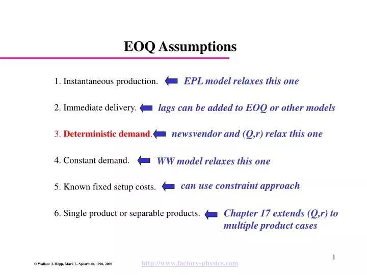
EOQ Assumptions. EPL model relaxes this one. 1. Instantaneous production. 2. Immediate delivery. 3. Deterministic demand . 4. Constant demand. 5. Known fixed setup costs. 6. Single product or separable products. lags can be added to EOQ or other models. newsvendor and (Q,r) relax this one.

E N D
EOQ Assumptions EPL model relaxes this one 1. Instantaneous production. 2. Immediate delivery. 3.Deterministic demand. 4. Constant demand. 5. Known fixed setup costs. 6. Single product or separable products. lags can be added to EOQ or other models newsvendor and (Q,r) relax this one WW model relaxes this one can use constraint approach Chapter 17 extends (Q,r) to multiple product cases
Modeling Philosophies for Handling Uncertainty 1. Use deterministic model – adjust solution - EOQ to compute order quantity, then add safety stock - deterministic scheduling algorithm, then add safety lead time 2. Use stochastic model - news vendor model - base stock and (Q,r) models - variance constrained investment models
The Newsvendor Approach • Assumptions: 1. single period 2. random demand with known distribution 3. linear overage/shortage costs 4. minimum expected cost criterion • Examples: • newspapers or other items with rapid obsolescence • Christmas trees or other seasonal items • capacity for short-life products
Newsvendor Model • Cost Function:
Newsvendor Model (cont.) • Optimal Solution: taking derivative of Y(Q) with respect to Q, setting equal to zero, and solving yields: • Notes: Critical Ratio is probability stock covers demand 1 G(x) Q*
Multiple Period Problems • Difficulty: Technically,Newsvendor model is for a single period. • Extensions: ButNewsvendor model can be applied to multiple period situations, provided: • demand during each period is iid, distributed according to G(x) • there is no setup cost associated with placing an order • stockouts are either lost or backordered • Key: make sure co and cs appropriately represent overage and shortage cost.
Example • Scenario: • GAP orders a particular clothing item every Friday • mean weekly demand is 100, std dev is 25 • wholesale cost is $10, retail is $25 • holding cost has been set at $0.5 per week (to reflect obsolescence, damage, etc.) • Problem: how should they set order amounts?
Example (cont.) • Newsvendor Parameters: c0 = $0.5 cs = $15 • Solution: Every Friday, they should order-up-to 146, that is, if there are x on hand, then order 146-x.
Newsvendor Takeaways • Inventory is a hedge against demand uncertainty. • Amount of protection depends on “overage” and “shortage” costs, as well as distribution of demand. • If shortage cost exceeds overage cost, optimal order quantity generally increases in both the mean and standard deviation of demand.
The (Q,r) Approach • Assumptions: 1. Continuous review of inventory. 2. Demands occur one at a time. 3. Unfilled demand is backordered. 4. Replenishment lead times are fixed and known. • Decision Variables: • Reorder Point:r – affects likelihood of stockout (safety stock). • Order Quantity:Q – affects order frequency (cycle inventory).
Inventory vs Time in (Q,r) Model Inventory Q r l Time
Base Stock Model Assumptions • 1. There is no fixed cost associated with placing an order. • 2. There is no constraint on the number of orders that can be placed per year.
Base Stock Notation • Q = 1, order quantity (fixed at one) • r = reorder point • R = r +1, base stock level • l = delivery lead time • q = mean demand during l • = std dev of demand during l • p(x) = Prob{demand during lead time lequals x} • G(x) = Prob{demand during lead time l is less than x} • h = unit holding cost • b = unit backorder cost • S(R) = average fill rate (service level) • B(R) = average backorder level • I(R) = average on-hand inventory level