Download
1 / 55
550 likes | 899 Views
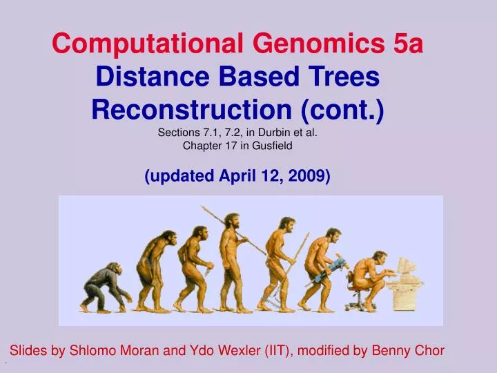
Computational Genomics 5a Distance Based Trees Reconstruction (cont.) Sections 7.1, 7.2, in Durbin et al. Chapter 17 in Gusfield (updated April 12, 2009) Slides by Shlomo Moran and Ydo Wexler (IIT), modified by Benny Chor Evolution Evolution of new organisms is driven by Diversity

E N D
Computational Genomics 5a Distance Based Trees Reconstruction (cont.) Sections 7.1, 7.2, in Durbin et al.Chapter 17 in Gusfield(updated April 12, 2009) Slides by Shlomo Moran and Ydo Wexler (IIT), modified by Benny Chor .
Evolution Evolution of new organisms is driven by • Diversity • Different individuals carry different variants of the same basic blue print • Mutations • The DNA sequence can be changed due to single base changes, deletion/insertion of DNA segments, etc. • Selection bias
The Tree of Life Source: Alberts et al
Tree of life- a better picture D’après Ernst Haeckel, 1891
Primate evolution A phylogeny is a tree that describes the sequence of speciation events that lead to the forming of a set of current day species; also called a phylogenetic tree.
Historical Note • Until mid 1950’s phylogenies were constructed by experts based on their opinion (subjective criteria) • Since then, focus on objective criteria for constructing phylogenetic trees • Thousands of articles in the last decades • Important for many aspects of biology • Classification • Understanding biological mechanisms
Morphological vs. Molecular • Classical phylogenetic analysis: morphological features: number of legs, lengths of legs, etc. • Modern biological methods allow to use molecular features • Gene sequences • Protein sequences • Analysis based on homologous sequences (e.g., globins) in different species
Topology based on Morphology Bonobo Chimpanzee Man Gorilla Sumatran orangutan Bornean orangutan Common gibbon Barbary ape Baboon White-fronted capuchin Slow loris Tree shrew Japanese pipistrelle Long-tailed bat Jamaican fruit-eating bat Horseshoe bat Little red flying fox Ryukyu flying fox Mouse Rat Glires Vole Cane-rat Guinea pig Squirrel Dormouse Rabbit Pika Pig Hippopotamus Sheep Cow Alpaca Blue whale Fin whale Sperm whale Donkey Horse Indian rhino White rhino Elephant Carnivora Aardvark Grey seal Harbor seal Dog Cat Asiatic shrew Insectivora Long-clawed shrew Small Madagascar hedgehog Hedgehog Gymnure Mole Armadillo Xenarthra Bandicoot Wallaroo Opossum Platypus (Based on Mc Kenna and Bell, 1997) Archonta Ungulata
From Sequences to a Phylogenetic Tree Rat QEPGGLVVPPTDA Rabbit QEPGGMVVPPTDA Gorilla QEPGGLVVPPTDA Cat REPGGLVVPPTEG Different genes/proteins may lead to different phylogenetic trees
From sequences to a phylogenetic tree Rat QEPGGLVVPPTDA Rabbit QEPGGMVVPPTDA Gorilla QEPGGLVVPPTDA Cat REPGGLVVPPTEG There are many possible types of sequences to use (e.g. mitochondrial vs. nuclear proteins).
Perissodactyla Donkey Horse Carnivora Indian rhino White rhino Grey seal Harbor seal Dog Cetartiodactyla Cat Blue whale Fin whale Sperm whale Hippopotamus Sheep Cow Chiroptera Alpaca Pig Little red flying fox Ryukyu flying fox Moles+Shrews Horseshoe bat Japanese pipistrelle Long-tailed bat Afrotheria Jamaican fruit-eating bat Asiatic shrew Long-clawed shrew Mole Small Madagascar hedgehog Xenarthra Aardvark Elephant Armadillo Rabbit Lagomorpha + Scandentia Pika Tree shrew Bonobo Chimpanzee Man Gorilla Sumatran orangutan Primates Bornean orangutan Common gibbon Barbary ape Baboon White-fronted capuchin Rodentia 1 Slow loris Squirrel Dormouse Cane-rat Rodentia 2 Guinea pig Mouse Rat Vole Hedgehog Hedgehogs Gymnure Bandicoot Wallaroo Opossum Platypus Topology1 , based on Mitochondrial DNA (Based on Pupko et al.,)
Chiroptera Round Eared Bat Eulipotyphla Flying Fox Hedgehog Pholidota Mole Pangolin Whale 1 Cetartiodactyla Hippo Cow Carnivora Pig Cat Dog Perissodactyla Horse Rhino Glires Rat Capybara 2 Scandentia+ Dermoptera Rabbit Flying Lemur Tree Shrew 3 Human Primate Galago Sloth Xenarthra 4 Hyrax Dugong Elephant Afrotheria Aardvark Elephant Shrew Opossum Kangaroo Topology2 ,based on Nuclear DNA (Based on Pupko et al. slide) (tree by Madsenl)
Theory of Evolution • Basic idea • speciation events lead to creation of different species. • Speciation caused by physical separation into groups where different genetic variants become dominant • Any two species share a (possibly distant) common ancestor
Aardvark Bison Chimp Dog Elephant Phylogenenetic trees • Leafs - current day species • Nodes - hypothetical most recent common ancestors • Edges length - “time” from one speciation to the next
Types of Trees A natural model to consider is that of rooted trees Common Ancestor
Types of trees Unrooted tree represents the same phylogeny without the root node Depending on the model, data from current day species often does not distinguish between different placements of the root.
Tree a Tree b Rooted versus unrooted trees Tree c b a c Represents all three rooted trees
Number of Different Trees on n Leaves For n=4, there are 3 different unrooted trees For n=5, there are 3*5=15 different unrooted trees For n=6, there are 3*5*7=15 different unrooted trees For n, there are n!! = 3*5*…*(2n-5)=(2n-5)!/[2n-3 *(n-3)!] different unrooted trees on n labeled leaves. There are 3*5*…*(2n-3)=(2n-3)!/[2n-2 *(n-2)!] different rooted trees on n labeled leaves (same as number of unrooted trees on n+1 labeled leaves. In both cases, number is too large to go over all of them!
Positioning Roots in Unrooted Trees • We can estimate the position of the root by introducing an outgroup: • a set of species that are definitely distant from all the species of interest Proposed root Falcon Aardvark Bison Chimp Dog Elephant
Phylogenetic Trees - Methods • There are several methods with which we construct trees and estimate how good a tree describes the data (and thus the evolution process) • Distance based methods • Parsimony • character based methods • Likelihood • Whole genome/proteome methods
Methods • Distance-based • Input is a matrix of distances between species. • Can be fraction of residue they disagree on, or alignment score between them, etc. • Character-based • Input is a multiple sequence alignment. Sequences consist of characters (e.g., residues) that are examined separately. • Genome/Proteome –based • Input is whole genome or proteome sequences. • No MSA or obvious distance definition.
Tree Construction: Different Outcomes • Distance Based- Output is a weighted tree that realizes the distances between the objects (or gets close to it). • Character Based – Output is a tree that optimizes an objective function based on all characters in input sequences (major methods are parsimony and likelihood). We start with distance based methods, and consider the following question: Given a set of species (leaves in a supposed tree), and distances between them – construct a phylogeny which best “fits” the distances.
Exact solution: Additive sets Given a set M of L objects with an L×Ldistance matrix: • d(i,i)=0, and for i≠j, d(i,j)>0 • d(i,j)=d(j,i). • For all i,j,k it holds that d(i,k) ≤ d(i,j)+d(j,k). Can we construct a weighted tree which realizes these distances? We should first clarify what realizes means.
Additive sets (cont) We say that the set of distances M on L objects is additive if there is a tree T, L of its nodes correspond to the L objects, with positive weights on the edges, such that for all i,j, d(i,j) = dT(i,j), the length of the path from i to j in T. Note: Sometimes the tree is required to be binary, and then the edge weights are required to be just non-negative.
k c b j m a i Three objects sets is always additive: For L=3: There is always a (unique) tree with one internal node. 3 equations in 3 unknowns: a,b,c Thus
How about four objects? L=4: Not all sets with 4 objects are additive: e.g., there is no tree which realizes the distances below.
k i l j The Four Points Condition Theorem: A set M of L objectsis additive iff any subset of four objects can be labeled i,j,k,l so that: d(i,k) + d(j,l) = d(i,l) +d(k,j) ≥ d(i,j) + d(k,l) We call (i,j),(k,l) the “split” of {i,j,k,l}. Proof: Additivity 4 Points Condition: By the figure (and maybe the board...)
Additive Distances We say that a distance metric D on L objects is additive if there is an unrooted binary tree on L leaves, with positive edge weights, that realizes the distanceD. Namely for all i,j, D(i,j)=DT(i,j)
Characterizing Additive Distances Thm: Any additive distance is fully characterized by the four point condition: Any 4 points can be renamed such that
7 C A Trees from Additive Distances: Algorithm • Verify that the distance matrix constitutes an additive metric • Choose a pair of objects, which results in the first path in the tree. • Choose a third object and establish the linear equations to let the object branch off the path. • Choose a pair of leaves in the tree constructed so far and compute the point a newly chosen object is inserted at. • 1. If the new path branches off an existing branch in the tree: Do the insertion step once more, replacing one of the two original leaves by another leaf along the branching path. • 2. Once the new path branches off an edge in the tree, this insertion is finished.
Trees from Additive Distances: Algorithm • Verify that the distance matrix constitutes an additive metric • Choose a pair of objects, which results in the first path in the tree. • Choose a third object and establish the linear equations to let the object branch off the path. • Choose a pair of leaves in the tree constructed so far and compute the point a newly chosen object is inserted at. • 1. If the new path branches off an existing branch in the tree: Do the insertion step once more, replacing one of the two original leaves by another leaf along the branching path. • 2. Once the new path branches off an edge in the tree: This insertion is finished. A 1 6 C X 1 B
Trees from Additive Distances: Algorithm • Verify that the distance matrix constitutes an additive metric • Choose a pair of objects, which results in the first path in the tree. • Choose a third object and establish the linear equations to let the object branch off the path. • Choose a pair of leaves in the tree constructed so far and compute the point a newly chosen object is inserted at. • 1. If the new path branches off an existing branch in the tree: Do the insertion step once more, replacing one of the two original leaves by another leaf along the branching path. • 2. Once the new path branches off an edge in the tree: This insertion is finished. d(A,B)=d(A,X)+d(X,B) d(A,C)=d(A,X)+d(X,C) d(B,C)=d(B,X)+d(X,C)
Trees from Additive Distances: Algorithm • Verify that the distance matrix constitutes an additive metric • Choose a pair of objects, which results in the first path in the tree. • Choose a third object and establish the linear equations to let the object branch off the path. • Choose a pair of leaves in the tree constructed so far and compute the point a newly chosen object is inserted at. • 1. If the new path branches off an existing branch in the tree: Do the insertion step once more, replacing one of the two original leaves by another leaf along the branching path. • 2. Once the new path branches off an edge in the tree: This insertion is finished. A 1 6 C X 1 B
Trees from Additive Distances: Algorithm • Verify that the distance matrix constitutes an additive metric • Choose a pair of objects, which results in the first path in the tree. • Choose a third object and establish the linear equations to let the object branch off the path. • Choose a pair of leaves in the tree constructed so far and compute the point a newly chosen object is inserted at. • 1. If the new path branches off an existing branch in the tree: Do the insertion step once more, replacing one of the two original leaves by another leaf along the branching path. • 2. Once the new path branches off an edge in the tree: This insertion is finished. C 5 A 1 1 1 2 B D (we now add E on the A-to-D path)
Trees from Additive Distances: Algorithm • Verify that the distance matrix constitutes an additive metric • Choose a pair of objects, which results in the first path in the tree. • Choose a third object and establish the linear equations to let the object branch off the path. • Choose a pair of leaves in the tree constructed so far and compute the point a newly chosen object is inserted at. • 1. If the new path branches off an existing branch in the tree: Do the insertion step once more, replacing one of the two original leaves by another leaf along the branching path. • 2. Once the new path branches off an edge in the tree: This insertion is finished. C 5 A 1 1 E 5 1 2 B NO! D
Trees from Additive Distances: Algorithm • Verify that the distance matrix constitutes an additive metric • Choose a pair of objects, which results in the first path in the tree. • Choose a third object and establish the linear equations to let the object branch off the path. • Choose a pair of leaves in the tree constructed so far and compute the point a newly chosen object is inserted at. • 1. If the new path branches off an existing branch in the tree: Do the insertion step once more, replacing one of the two original leaves by another leaf along the branching path. • 2. Once the new path branches off an edge in the tree: This insertion is finished. E 3 A 2 1 1 3 C 1 2 B D
Trees from Additive Distances: Algorithm is this necessary? • Verify that the distance matrix constitutes an additive metric • Choose a pair of objects, which results in the first path in the tree. • Choose a third object and establish the linear equations to let the object branch off the path. • Choose a pair of leaves in the tree constructed so far and compute the point a newly chosen object is inserted at. • 1. If the new path branches off an existing branch in the tree: Do the insertion step once more, replacing one of the two original leaves by another leaf along the branching path. • 2. Once the new path branches off an edge in the tree: This insertion is finished. E 3 A 2 1 1 3 C 1 2 B D
Reconstructing a Tree from an Additive Distance By algorithm, given a distance matrix constituting an additive metric, the topology of the corresponding additive tree is unique. Q.: Given an additive metric on n leaves, what is the run time of the algorithm? A.: Number of phases is n. Work per phase is O(n). So total is O(n2). E 3 A 2 1 1 3 C 1 2 B D
Approximating Additive Metrices In practice, the distance matrix between molecular sequences will not be additive. In such case we want to find a tree T whose distance matrix is “close” to the given one. The methods for exact tree reconstruction provide an inventory for heuristics for tree construction based on approximating additive metrics. Heuristics give exact results when operating on additive metrics, but the performance of solutions gets unclear when non additive metrics are handled.
A B C D Neighbor Finding How can we find from distances alone a pair of sisters (neighboring leaves)? Important observation: Closest nodes are not necessarily neighboring leaves. Next, we show a way to find neighbors from distances. The method is simple, but unfortunately not very intuitive
Neighbour Joining Algorithm: Outline • Identifya pair of leaves u,v asneighbors. • Combineu,v into a new node, w. • Update the distance matrix: Calculate w’s distance from • any other node x of the tree using • Notice that all 3 quantities on rhs are known. • When only 3 nodes are left – compute 3 distances & finish.
i m 0.1 0.1 0.1 k l 0.4 0.4 j n Neighbour Joining Algorithm • Identify a pair of neighborsi,j among n leaves. • Combine i,j into a new node u. • Update the distance matrix. • When only 3 nodes are left – finish. Let ri be the sum of distances from i to every other node The measure between i and j we use in the algorithm is
i m 0.1 0.1 0.1 k l 0.4 0.4 j n Neighbour Joining Algorithm Let ri be the sum of distances from i to all other nodes The measure between i and j we use in the algorithm is
T1 T2 m l k i j Neighbor Finding: Seitou & Nei method Theorem (Saitou&Nei)Assume D is additive, and all tree edge weights are positive. If XD(i,j) is minimal (among all pairs of leaves), then iandj are sister taxa in the tree. The proof is rather involved, and will be skipped (no tears, pls).
m k i j Complexity of Neighbor Joining Algorithm Naive Implementation: Initialization:θ(L2) to compute the XD(i,j)’s. Each Iteration: • O(L) to update {XD(i,k):i L} for the new node k. • O(L2) to find the minimalXD(i,j). Total of O(L3). • This can be improved using better data structures (e.g. heap)
Reconstructing Trees from Additive Matrices • Q: Do we have to test additivity before running NJ? • A: By Seito-Nei, if matrix is additive, NJ will constructthe correct tree. Algorithm does not care about awareness and need not know anything about the matrix! E 3 A 2 1 1 3 C 1 2 B D
U B Running NJ: Example on 4 Leaves A Remark: The XD values imply that the distances are not additive (why?).
U B Updated Distance Matrix,Choosing A,B as Neighbors V d(U,x)=[d(A,x)+d(B,x)-d(A,B)]/2 D A Notice that now we have only one Choice: The neighbors are U and D.
U B Final Distance Matrix V C D A Remark: Resulting tree is unrooted.
Reconstructing Trees from non Additive Matrices Q: What if the distance matrix is not additive? A: We could still run NJ (like we just did)! Q: But can anything be said about the resulting tree? A: Not really.Resulting tree topology could even vary according to way ties are resolved on the way. Remark: This indeed was the case with last example.