Journal of Physics & Astronomy

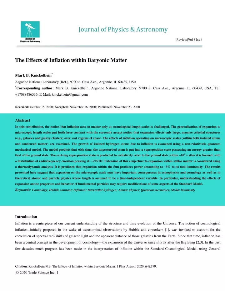
Journal of Physics & Astronomy Review|Vol 8 Iss 4 The Effects of Inflation within Baryonic Matter Mark B. Knickelbein* Argonne National Laboratory (Ret.), 9700 S. Cass Ave., Argonne, IL 60439, USA *Corresponding author: Mark B. Knickelbein,Argonne National Laboratory, 9700 S. Cass Ave., Argonne, IL 60439, USA, Tel: +17088486536; E-Mail: knickelbein@gmail.com Received: October 15, 2020; Accepted: November 16, 2020; Published: November 23, 2020 Abstract In this contribution, the notion that inflation acts on matter only at cosmological length scales is challenged. The generalization of expansion to microscopic length scales put forth here contrast with the currently accept notion that expansion effects only large, massive celestial structures (e.g., galaxies and galaxy clusters) over vast regions of space. The effects of inflation operating on microscopic scales (within both isolated atoms and condensed matter) are examined. The growth of isolated hydrogen atoms due to inflation is examined using a non-relativistic quantum mechanical model. The model predicts that with time, the unperturbed atom is put into a superposition state possessing an energy greater than that of the ground state. The evolving superposition state is predicted to radiatively relax to the ground state within ~105 s after it is formed, with a distribution of radiofrequency emission peaking at ∼ ∼275 Hz. Extension of this conjecture to expansion within stellar matter is considered using a thermodynamic analysis. It is predicted that expansion within the Sun produces power amounting to ~3% to its total luminosity. The results presented here suggest that expansion on the microscopic scale may have important consequences in astrophysics and cosmology as well as in theoretical atomic and particle physics where length is assumed to be a time-independent variable. In particular, understanding the effects of expansion on the properties and behavior of fundamental particles may require modifications of some aspects of the Standard Model. Keywords:Cosmology; Hubble constant; Inflation; Interstellar hydrogen; Atomic physics; Quantum mechanics; Stellar luminosity Introduction Inflation is a centerpiece of our current understanding of the structure and time evolution of the Universe. The notion of cosmological inflation, initially proposed in the wake of astronomical observations by Hubble and coworkers [1], was invoked to account for the correlation of spectral red- shifts of galactic light and the apparent distance of those galaxies from the Earth. Since that time, inflation has been a central concept in the development of cosmology—the expansion of the Universe since shortly after the Big Bang [2,3]. In the past few decades much progress has been made in the interpretation of inflation within the Standard Cosmological Model, using General Citation: Knickelbein MB. The Effects of Inflation within Baryonic Matter. J Phys Astron. 2020;8(4):199. © 2020 Trade Science Inc. 1

www.tsijournals.com | November-2020 Relativity as a theoretical framework [4-8]. The basic notion of exponential spatial inflation has stood the test of time and is now central to our understanding of the Big Bang and its aftermath in the evolution of the Universe. The exponential expansion observed in the Universe is most commonly described by the Hubble–Lemaître law (commonly known as the Hubble Law), as parametrized by the Hubble Constant, H0 [6]. The value of the Hubble constant H0 is being constantly refined as experimental techniques and analysis methods improve, and there is currently some discrepancy between values determined using different approaches [9]. However, these discrepancies are of the order of only ~10 percent, and since the precise value of H0 is not important to the general conclusions gleaned from the following analyses, we shall use the most recently accepted value [6]: H0 = 68 ± 2 km s-1 Mpc-1 In discussing inflation at microscopic length scales, it is more convenient to use the rate constant form of the Hubble constant containing no reference to a particular length: H0 = 6.95 × 10-2 Gyr-1 H0 =2.20 × 10-18 s-1 Any length l of space is then predicted to expand exponentially with time as, ( ) ( ) -1 = 14.4 × 109 years—a value not far from the estimated age of the Universe since the Big Note that when H0 is expressed in this way, H0 Bang: ~13.8 × 109 years [3]. If, we accept that the ―fabric‖ of space is continuous at every length scale, then it becomes interesting to consider the effects of inflation at the microscopic level, in particular how inflation effects the internal structure of isolated atoms and other baryonic matter in the Universe. Hydrogen is estimated to make up >90% of the baryonic matter of the Universe [4,10]. The majority of hydrogen is contained in the interstellar-and intergalactic media, some as neutral hydrogen atoms, some as ionized hydrogen—bare protons (p) and electrons (e) in low- density plasmas [11]. In the intergalactic medium, the density of hydrogen is estimated to be of the order of one atom (or proton) per cubic meter. At this density, the mean time between collisions (H-H, H-p, H-He, p-e, etc.) is ~107-109 years, varying with the density and temperature of the medium, and the collision partner. (A gas kinetics approach that can be used to make simple mean-time-between- collision estimates is outlined in the Appendix.) Neutral hydrogen atoms in the intergalactic environment are thus relatively unperturbed on the timescale of the estimated age of the universe, ~1.4 × 1010 yr [3]. Because the effects of inflation on microscopic systems have not (to the author’s knowledge) been considered previously, we must improvise using the theoretical tools available. In the following analysis, we consider the effects of inflation on the internal space within the isolated hydrogen atom using the methods of non-relativistic quantum mechanics. We then consider the effects of inflation within the dense matter comprising stellar interiors using a classical thermodynamical model. 2

www.tsijournals.com | November-2020 Expansion within the hydrogen atom The notion that the empty space within microscopic baryonic matter expands with time is conceptual terra incognita. So, we can only proceed with a theoretical analysis of this phenomenon using the tools we have available. In the case of the isolated hydrogen atom, we will use well-established methods of quantum mechanics. The hydrogen atom in its ground state has a volume of ∼10-31 m3, using the Bohr radius, a0 (= 0.0529 nm), as an approximate (but well- defined) measure of its size. In contrast, the volume of hydrogen’s nucleus, the proton, is ∼10-45 m3, while the electron, a lepton has, in comparison, no (or negligible) volume. Thus, the hydrogen atom is almost entirely made up of empty space. The expansion of the internal volume of the hydrogen atom with time will be treated assuming that the Hubble expansion law is valid at atomic length scales. With the assumption of exponential spatial expansion as given in Equation 1, the radius of the hydrogen atom R initially at R0 will then increase exponentially with time, like any other distance of space: ( ) ( ) Because the hydrogen atom in its ground (1s) state has no well-defined radius in the classical sense, we can simply assign R0 to the value of the Bohr radius, a0, or to the quantum mechanical expectation value of the proton-to-electron distance <r>1s = 3a0/2. The assignment of any precise value for its radius is not critical for this discussion, so in the following analysis we shall simply equate R0 to a0. Equation 2 predicts that, in the absence of external perturbations, the hydrogen atom’s radius (however it is defined) would increase by about 7% and its volume by about 23% in 109 years (1 Gyr). This growth conjecture, based on Equation 2, predicts that unperturbed hydrogen atoms will simply grow exponentially without bound; however this notion is not consistent with the true nature of atoms, which are properly described by quantum mechanics. In particular, the electron radial probability density of the hydrogen atom in its ground and excited states are well- understood within quantum mechanical theory, defined by the appropriate wave functions, and are not subject to arbitrary ―adjustment‖. Here, we use the non-relativistic formulation. To put intra-atom expansion of hydrogen on a firmer theoretical footing, we first cast the problem in classical form, in which we take a0 to be the initial radius of the normal ground-state atom. The energy of the ground state E0 is given by ( ) ( ) where E0 = -13.6 eV [12]. Increasing the internal volume of the atom amounts to increasing the mean proton-to-electron distance r from its most probable value ground-state value, a0, to an incrementally larger value a´. This radial expansion is accompanied by an incremental increase of potential energy ΔEV, given as the difference in Coulombic attraction: ( ) Using the tools of time-independent perturbation theory [13,14], the corresponding energy perturbation term in the Hamiltonian, Ĥ´, contains only a´ and a0, with no (differential) quantum mechanical operators, and is thus identical in form to the classical expression, Equation 4, 3

www.tsijournals.com | November-2020 ( ) Using the exact ground state wave function for the hydrogen atom, ψ1s, we then calculate the first-order correction EV= <ψ1s |Ĥ´| ψ1s> to the ground state energy E0. Using the perturbation Hamiltonian given by Equation 5, the first order energy correction EV is given as ( ) The perturbation theory result given by Equation 6 is found to be identical to the classical result given by Equation 4, except reversed in sign reflecting the addition of energy upon increasing the atom’s radius (EV is a positive quantity). Thus, the effect of expansion is to add energy to the atom due to the increased potential energy of the expanded system. The time-evolution of the added energy EV(t) is found by substituting the growth expression for a´ in Equation (6): ) ( ) ( -1, giving the total energy Etot = E0 + EV for the atom: Equation (7) predicts that as t→∞, EV approaches a0 ( ) ( ) The asymptotic value for Etot given by Equation 8b is +13.6 eV, clearly at odds with the expected total energy for infinite proton-electron separation, 0 eV. The discrepancy can be traced to the neglect of the electron’s kinetic energy T in the analysis: the total energy Etot must approach zero as the potential energy EV approaches its maximum at infinite separation. The quantum mechanical virial theorem, as applied to the hydrogen atom, predicts that the expectation values of the potential energy <V> and kinetic energy <T> are related to the total energy Etot as follows [13,14]: ( ) ( ) Thus, ( ) Following this result, we reformulate an expression for Etot that accounts for the electron kinetic energy, adapting the virial theorem to account for the changes in T and V as the atom expands: ( ) ( ) ( ) 4

www.tsijournals.com | November-2020 ) ) ( ) ( ( ( ) In Equations 10a and 10b, the first term is the total ground-state energy of the unexpanded atom, the second term is the change in potential energy EV(t), and the third term is the change in kinetic energy ET(t) (= -EV(t)/2) obtained using the virial theorem adaptation. With this modification, Etot exhibits the expected asymptotic behavior as t→∞: ( ) ( ) ( ) ( ) The time evolution of Etot as predicted by Equation 10c is shown in (FIG. 1). Also shown in (FIG. 1) are the computed expectation values <r>1s, <r>2s, <r>3s, and <r>4s along with the experimental energies for those states. Note that the Etot curve passes smoothly through the well-established energy eigenvalues corresponding to the <r>ns. FIG. 1. Total energy of the hydrogen atom as a function of time, as predicted by Equation (9). The top axis shows the corresponding size of the atom as a function of <r>/a0. The solid circles are the <r>ns and Ens (= E0n-2) values computed for n = 1-4. The quantum mechanical treatment applied here gives us a simple picture of the hydrogen atom that becomes incrementally inflated with time, but does not address its ultimate fate. This analysis predicts unlimited exponential expansion, but that is physically unrealistic. In our 5

www.tsijournals.com | November-2020 model of isotropic (spherical) expansion, the mean proton-to-electron distance <r> would seem to increase without bound. However, the excited states with n>1 would eventually interrupt the expansion by providing a means to return to the ground state via dipole-allowed transitions. In particular, when <r> in our expanding atom approaches that of the 2 s state (<r>2s = 6a0), the atom would be expected to return to the ground state by emission of an ultraviolet photon, via the Lyman-α transition (λ = 121.6 nm; hυ = 10.2 eV) [12]. The time t2s required for the atom to increase in size from the ground 1 s state to the 2 s state (as measured by <r>2s) is calculated to be ~19.9 Gyr— greater than the estimated age of the Universe. But, how do we describe these atoms between 1 s and 2 s? To address this, we turn again to the available tools: the quantum mechanics and spectroscopy of time-dependent systems. A hydrogen atom that has become expanded in volume, even incrementally, is clearly no longer in its ground state, but rather must be described quantum mechanically as a (time-dependent) superposition state Ψ(t) [13,14]. The contribution of the excited (n>1) states to this state increases continuously as the dimensions of the atom increases with time. Formally, we express the electronic structure of this superposition state as of a linear combination of the ground and excited states of hydrogen: ( ) ( ) ( ) ∑ where ψns are the ground (n = 1) and excited (n≥ 2) s-state wave functions. Note that the expansion coefficients cn are, in general, complex and time-dependent. Atomic hydrogen 2 s-1s superposition states have in fact been produced in the laboratory, in ultrafast laser excitation experiments [15]. However in these experiments, their existence is fleeting, so their properties cannot be studied in detail. Because the expansion of space within the atom is assumed to be isotropic, and because there is assumed to be is no mechanism for change of angular momentum for the isolated atom (so as to produce states of non-zero angular momentum: p, d, f…), we consider only the hydrogenic s states in the linear combination (Equation 12), thus preserving the spherical symmetry of the atom. In this simple picture, the effect of spatial expansion is to contribute excited s states into overall wave function Ψ(t). Because this superposition state contains contributions of excited s states, there must exist a nonzero probability for dipole-allowed transitions to the ground state that increases with the fraction of excited-state character in the inflated atom that is as the atom increases in size. We therefore consider the dynamical properties of these superposition states Ψ(t). Because nothing is known about the dynamical (e.g., radioactive) properties of superposition states in atomic hydrogen, we will first simplify the problem by initially only considering the 1 s and 2 s states, but with the implicit understanding that all ns states actually contribute to the superposition state, as given by Equation 12. In this simplified model, we will denote the 2s-1s superposition state as: ( ) ( ) ( ) ( ) Whereas the (complex) coefficients cn(t) give the contribution of each basis wave function ψns in the overall wave function Ψ(t), it is the |cn|2 (= cncn *) terms that provide the connection to the physical observables such as electron probability density and radioactive properties [13,14]. The cn(t) then must satisfy the following criteria: 6

www.tsijournals.com | November-2020 1. Following our physical description of the growth of the atom (see above), [c2(t)]2must increase exponentially from 0→1 as t varies from 0→t2s, where t2s = 6.28 × 1017 s (19.9 Gyr). That is, at t2s = 6.28 × 1017 s, the atom reaches the dimensions of the 2s state, which is a factor of 4 larger than the ground state (<r>2s/<r>1s = 4) 2. [c1(t)]2 must decrease with time as c1(t) varies from 1 at t = 0 to 0 at t = t2s 3. Completeness must be satisfied: |c1(t)2| + |c2(t)2| = 1 Using criterion 1, it is readily shown that ( ) ( ) ( ) satisfies these requirements between t = 0 and t = t2s. Then, by the completeness requirement (Criterion 3), [c1(t)]2 = 1-[c2(t)]2 Now, proceeding further into terra incognita, we must make some assumptions regarding the radiative properties of the superposition state, in particular how its radiative decay rate varies with the composition of Ψ(t) at any given t. We begin by defining a first-order, time- dependent rate coefficient, k21(t), that describes the emission rate of the 2s-1s superposition state given by the decay rate of the ―inflated‖ population. Lacking any available theoretical model to guide us in this problem, we will simply assume that k21(t) varies in proportion to the square of the fraction of ψ2sin Ψ(t): k21(t) ~ [c2(t)]2 (Equation 13). The radiative decay rate (τ-1) of the pure 2 s state, A21, is 4.70 × 108 s-1 for the Lyman-α (2s→1s) transition [12]. Because k21(t) is assumed to vary from 0 for the atom in its 1s ground state at t = 0, to A21 at t = t2s when the atom has reached the 2 s state, it follows that k21(t)=[c2(t)]2A21. From Equation 14 it is seen that for small t, [c2(t)]2 = H0t/3. Thus, in the small t limit, k21(t) ≅ A21H0t/3 In the following analysis, we shall see that the assumption of small t (t<<t2s) is justified. The emission spectrum generated by radiative decay of the superposition state Ψ(t) is calculated using a rate equation approach, assuming an initial population N(0) of ground state hydrogen atoms at t = 0. We redefine the zero of energy to be that of the ground state, so that E(0) = 0 and ( ) ( ) The emission spectrum is defined by the radiative decay rate of the evolving population N(E) as a function of time (and energy): ( ) ( ) ( ) ( ) ( ) ( ) ( ) ( ) ( ( ) ) ( ) 7

www.tsijournals.com | November-2020 The time evolution of the emission intensity predicted by Equations 15a-15c is shown in (FIG. 2). The model predicts that the emission intensity peaks at ∼4 × 104 s, more than 12 orders-of-magnitude smaller than t2s itself. Thus, radiative decay dominates unlimited spatial growth, returning the ensemble of atoms to its original 1s ground by ∼2 × 105 s, at which point the growth process begins again. FIG. 2. The emission spectrum predicted for a population of hydrogen atoms born in their normal 1 s ground state at t=0. Red curve: Emission spectrum calculated assuming a superposition state contribution from 2 s only; Blue curve: Spectrum calculated assuming a superposition state contribution from 2 s, 3 s, 4 s, and 5 s states. Note that the emission frequencies of the inflating ensemble of atoms are time-dependent: the bottom axis shows the time dependence of the emission intensity; the top axis shows their emission frequencies. See Equations (12-14) for details of the model. For the radiative rate analysis thus far, we have truncated the superposition series given by Equation 12 and considered only the 2 s excited state in the derivation of the emission rate expression given by Equation 15a-15c. Inclusion of additional higher-lying ns states (n = 3, 4, 5…) in the analysis leads to additional rate coefficients kn1(t), each contributing to the overall emission rate to the ground state in parallel with k21. We define ktot as the sum of the individual rates: ktot = Σ kn1 (n = 2-∞) The rate expressions given by Equations 15a-15c thus provide a lower bound to ktot. Calculation of kn1 for n = 3-5 using the same analysis given above for n = 2 using the accepted An1 emission rates [12] show that these rate coefficients decrease rapidly with increasing n:k31 is a factor of 20 smaller than k21, while k41 is an order-of-magnitude smaller than k31, and so on. The emission spectrum calculated for ktot 8

www.tsijournals.com | November-2020 including the n = 2-5 excited states in the analysis is shown in FIG. 2, along with that calculated using only n = 2. Comparison of the two spectra shows only a small shift to lower emission times (and lower frequencies) when higher n states are included, confirming that k21 is the dominant term in ktot. The emission frequencies predicted with this model, also shown in FIG. 2, lie in lowest-energy portion of the radiofrequency region, many orders-of-magnitude lower than that of the Cosmic Microwave Background (CMB) and other galactic and extragalactic radiofrequency emissions that have been detected [16]. The predicted emission rate is sufficiently rapid that competition from collisional relaxation would not be a complicating factor, even for hydrogen in dense molecular clouds—including those within our own Galaxy [11]. Unfortunately, experimental verification of the predicted spectrum is not possible from Earth-based instruments because the predicted emission frequencies lie in the radiowave-opaque region of the RF spectrum, where radiation does not penetrate the ionosphere [16]. Thus, space- based probes incorporating the appropriate instrumentation would be required to detect the ultralow-frequency RF emissions predicted in this analysis. Expansion within condensed matter Stars comprise the overwhelming majority (>99%) of the condensed matter in the known Universe [1]. The pressures within normal stars are enormous from our terrestrial point-of-view. The pressures within our Sun, for example, vary from ~1016 Pa at the center (r = 0) to ~1011 Pa at r = 0.9 R⊙, finally approaching zero at the surface, r = R⊙ [17]; the atmospheric pressure on Earth at sea-level is, by contrast, only ∼105Pa. However even at a normal star’s center, it is easily calculated that the constituent matter is largely ―empty space.‖ If we accept the idea that this empty space within the interior of the Sun and other stars expands at a linear rate H0, we are compelled to consider the energetic implications. In particular, we must devise a means to calculate the energetic consequences of space being continuously ―created‖ within the high-pressure environment of a star, due to inflation. While the creation of volume within condensed matter due to cosmological expansion has no classical analog, we nevertheless adapt a thermodynamic model here to describe this phenomenon. The creation of an increment of space within stellar matter due to expansion will produce a non-equilibrium expanded state, which is assumed to relax instantaneously. Given the large collision rate, the expansion-relaxation cycle will be so rapid that it would seem that at first glance that there should be no observable effect. However, this continuously-occurring process must be considered as a source of internal power to the star due to P-V work, adding to the power that is produced via fusion processes in the stellar core. To calculate this additional power source, we will proceed with a thermodynamic approach. The generalized integrated form of the Hubble expression describing expansion of any given initial length l0 initially at t = 0 is ( ) 3) is simply, (Equation 1), so that the expansion of any arbitrary volume V0 (= l0 ( ) ( ) The increment of P-V work dWP-V generated within volume dV at a pressure P(r) and at a distance r from the center of the star then is then, ( ) ( ) with the corresponding increment of power dPP-V given by, 9

www.tsijournals.com | November-2020 ( ) ( ) ( ) ( ) where Equation (18b) was obtained using the expression for V(t) given in Equation (16). Because it is assumed that relaxation of the non- equilibrium expanded state of stellar matter is instantaneous, we let t = 0 in Equations (18), and set the initial volume V0 to the spherical volume element at radius r: V0(r) = 4πr2dr Then, integrating the resulting expression over r, we obtain an expression for the total power PP-V: ( ) ∫ ( ) Our Sun, a typical star whose properties are as well-known as any, has a pressure profile P(r) predicted by the Standard Solar Model [17]. Using the tabulated values of P(r) vs. r obtained from this model, we evaluate PP-V by simple numerical integration of the integral on the rhs of Equation 19 and obtain the final result: PP-V= 1.3 × 1035 W. This amounts to 3.4% of the total luminosity of the Sun (L⊙≅3.8 × 1026 W) [18]. Thus, expansion is predicted to contribute to the power output of the Sun in a small (but non-negligible) way. Finally, it is noted that this same analysis would not apply to neutron stars, as they do not contain any significant ―empty space‖ within them for expansion to occur—they are thought to be composed of voidless, ―solid‖ baryonic matter (sometimes referred to as ―neutronium‖). Summary In this paper, the notion that the microscopic internal space within baryonic matter expands with time has been put forth. The author stresses that the analyses in this paper are by no means unique: they are simply best-effort calculations based on what we know as applied to what we do not. For isolated matter such as intergalactic atomic hydrogen, the internal expansion conjecture might be dismissed off- hand by invoking the occurrence of a relaxation mechanism, continuously acting to maintain the atom in its ground, uninflated state. With that assumption, space expands over time but atoms fly through it unaffected, forever displaying their original (ground) state internal dimensions (and energies). However, such continuous relaxation would require a medium to serve as a ―heat bath‖, and in the absence of such a medium there is no mechanism for mediated relaxation—the only relaxation mechanism(s) must be intrinsic to the atom as space expands within it. It was once thought that such a medium existed, necessary to support the propagation of electromagnetic waves through space. However, Michelson and Morley demonstrated the absence of such an ―ether‖, through their landmark interferometry studies. The ―stretching‖ of the high-energy photons present at the dawn of transparency in the very early Universe to the CMB that we observe now is an example of inflation acting to increase the wavelengths of photons (thus reducing their momenta and energies) over the course of time without any medium or other intervening third-body mechanisms. Can the same notion of dimensional stretching operate in isolated baryonic matter? 10

www.tsijournals.com | November-2020 Within condensed matter a heat bath is ―built in‖, in the form rapid collisions between particles, enabling the relaxation to equilibrium of any non-equilibrium state produced by internal expansion, as would occur in any fluid. The net result is heat production due to the P-V work done on the system. As applied to the Sun, the resulting heat production is predicted to amount to a few percent of its total luminosity. While this is a modest fraction of the total output of the Sun, perhaps power production due to expansion within darker (lower temperature) stars might contribute a larger fraction to their luminosities. Appendix In order to assess whether or not an atom in an excited state undergoes collisional relaxation to the ground state in a given time, we need to know the probability that the atom undergoes a deactivating collision with another atom (or molecule, proton, electron, etc) in that time. Assuming that the gases in interstellar and intergalactic media are at (local) thermodynamic equilibrium, we can calculate their collision rate constant kc and hence mean-time-between-collisions, using the well-established kinetic theory of gases [19]. In its simplest form, kc is given by the product of the mean relative velocity between any two atoms in the ensemble <vr> and the collision cross section σc: ( ) 2, where rc is the effective collision radius of the colliding pair. For H-H collisions, for The collision cross section σcis calculated as πrc example, we would reasonably estimate the collision radius as the radius of the H atom=0.0529 nm (the Bohr radius a0), in which case σc = 8.8 × 10-21 m2. The mean relative velocity <vr> of two colliding atoms within an ensemble at temperature T is given [19] by: ⟨ ⟩ ( ) ( ) where µ is the reduced mass of the colliding pair. For the case of H-H collisions, µ = 8.3 × 10-28 kg. For ease of calculation, Equation (A2) can be then expressed as σc = 4.2 × 104 T1/2 ms-1 for H-H collisions. The collision rate Rc experienced by a single H atom is given by ( ) where n is the number density of collision partners, here taken to be atomic hydrogen. Using this model it is calculated, for example, that in a gaseous medium in which the density of hydrogen is 1 m-3 and the temperature is 100 K, the collision rate experienced by one H atom Rc = 3.7 × 10-17 s-1 (~1.1 collision per Gyr) and the mean time between collision (Rc = 2.7 × 1016 s (~0.9 Gyr-1). One can easily extrapolate the calculation of Rc to other values of n and T by noting that Rc is proportional to n -1) and to √T. Likewise, σc for collision partners other than hydrogen atoms can be estimated using standard bimolecular collision models [19]. REFERENCES 1.Hubble EP. A Relation between distance and radial velocity among extra-galactic nebulae. Proc Natl Acad Sci. 1929;15:168-73. 11

www.tsijournals.com | November-2020 2.Choudhuri AR. Astrophysics for physicists. Cambridge University Press, Cambridge, UK, 1929. 3.Ryden B. Introduction to cosmology. 2nd edn. Cambridge University Press, Cambridge, UK, 2017. 4.Bartelmann M. The dark universe. Rev Mod Phys. 2010; 82:331-82. 5.Bassett BA, Tsujikawa S, Wands D. (2006). Inflation dynamics and reheating. Rev Mod Phys. 2006;76:537-89. 6.Jackson N. The hubble constant. Living Rev Relativ. 2015;18: 2-95. 7.Lidsey JE, Liddle AR, Kolb EW, et al. Reconstructing the inflation potential—An overview. Rev Mod Phys. 1997;69:373-410. 8.Turner MS, Tyson JA. Cosmology at the millennium. Rev Mod Phys. 1999;71:S145-64. 9.Wong KC, Suyu SH, Chen GC, et al. H0LiCOW–XIII. A 2.4 percent measurement of H0from lensed quasars: 5.3σ tension between early-and late-Universe probes. Mon Not R Astron Soc. 2020;498:1420-39. 10.Voit GM. Tracing cosmic evolution with clusters of galaxies. Rev Mod Phys. 2005;77:207-58. 11.Tielens AGGM. The molecular universe. Rev Mod Phys. 2013;85:1021-81. 12.Wiese WL, Fuhr JR. Accurate atomic transition probabilities for hydrogen, helium, and lithium. J Phys Chem Ref Data. 2009;38:565-719. 13.Levine IN. Quantum chemistry. 5th edn. Prentice Hall, New York, US, 2000. 14.Cohen TC, Diu B, Laloe. Quantum mechanics. F Wiley and Sons, New York, US, 1977. 15.Scrinzi A, Geissler M, Brabec T. Techniques for at to second pulse detection and the observation of electronic quantum motion. Laser Phys. 2001;11:169-73. 16.Condon JJ, Ransom SM. Essential radio astronomy. Princeton University Press, Princeton, New Jersey, US, 2016. 17.Bahcall JN, Ulrich RK. Solar models, neutrino experiments, and helioseismology. Rev Mod Phys. 1988;60:297-332. 18.Michelson AA, Morley EW. On the relative motion of the Earth and the luminiferous ether. Am J Sci. 1887;34:333-45. 19.Smith IWM. Kinetics and dynamics of elementary gas reactions. Butterworths, London, UK, 1980. 12

Journal of Physics & Astronomy